Part 1 – Introduction to Adversarial Machine Learning

Welcome to the first part of our blog series on Adversarial Machine Learning! In this series, we will explore the fascinating field of adversarial machine learning, its background, techniques for attacks, and strategies for defense. Let’s begin with an introduction to adversarial machine learning and its relevance in today’s landscape.
Introduction
The world has adopted deep learning and computer vision applications to build intelligent systems such as autonomous vehicles, smart devices like Amazon Echo, drones, robots, and defect detection systems in the manufacturing industry. Evolution of technology in deep learning systems has led to the adoption of machine learning and artificial intelligence technologies in domestic and industrial environments. The deployment of these applications in the real world is only possible if the deep learning models are accurate enough and fast enough to work in real time. For example, Tesla employs deep learning and computer vision to develop self-driving car applications involving object detection, traffic sign recognition, semantic segmentation, pedestrian tracking, lane detection. Antivirus and anti-malware software uses machine learning models to predict the behaviour of an adversary. Such security-critical systems need fast and highly accurate classifiers, object detectors, and segmentation models, since small errors can also be critical.
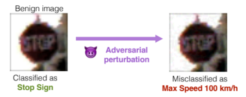
Unfortunately, machine learning models are susceptible to incorrect model classification when subjected to adversarial examples, despite the fact that they are expected to generalize to unseen data well in the real-world and be robust to anomalies and outliers. Adversarial attacks exploit overfitting of training data, under which any random noise added
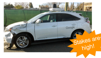
to the input data can cause the model to misclassify. Attackers can leverage this idea to craft adversarial examples and compromise machine learning models. Sensitive real world scenarios such as autonomous aircraft and self-driving cars can be severely compromised by real world adversaries employing these attacks.
In this blog series, we will delve into the world of adversarial machine learning, exploring different attack techniques like Fast Gradient Sign Method (FGSM), Projected Gradient Descent, Carlini and Wagner, AdvGAN, and more. We will also discuss defense strategies such as adversarial training, defensive distillation, and ensemble methods. Each topic will be accompanied by practical code examples to enhance your understanding and enable you to apply these concepts in real-world scenarios.
Pre-requisites
- Solid understanding of ML and deep learning concepts.
- Familiarity with PyTorch.
- A computer with a decent GPU or Colab/Kaggle workspace.
Generation of Adversarial Examples
To create an adversarial example, the goal is to minimize the adversarial attack algorithm’s objective while keeping the generated adversarial example to look as similar as possible to the original input.


Given a trained deep learning model f and an original input data sample x generating an adversarial example x′can generally be described as a box-constrained optimization problem:
\begin{align*}
\min_{x’} \|x’-x\| \\
\text{st. $f(x’)=l’$},\\
f(x)=l,\\
l\neq l’,\\
x’\in [0,1],
\end{align*}
\)
where \(l\) and \(l’\) denote the output label of \(x\) and \(x’\), \(|.|\) denote the distance between two data sample. Let \(\eta=x’-x\) be the perturbation added on \(x\).
In layman terms, the goal is to find the smallest possible perturbations that cause the network to make a mistake while keeping the changes imperceptible to human observers.
Distance Metrics
A practical attack would not only aim to fool the classifier but also create examples that are close to the original data. To achieve this, most attacks impose a distance constraint. Different distance metrics are used to quantify the dissimilarity between original input data and adversarial examples. The following are three most popular distance metrics.
- \(L_0\) is the total number of pixels that differ between the clean and perturbed image. (Zero-norm distance)
|\delta\|_1=\sum_{i=1}^{N}|\delta_i|
\)
- \(L_2\) is the squared difference between the pixel values of the clean and perturbed image. (Euclidean distance)
\|\delta\|_2=\sqrt{\sum_{i=1}^{N}\delta_i^2}
\)
- \(L_\infty\) is the maximum difference between the pixel values of the clean and perturbed image. (Max-norm or Chebyshev distance)
\|\delta\|_\infty=\max{\{|\delta_i|: i=1,…,N\}}
\)
The choice of distance metric depends on the specific application and the desired trade-off between the magnitude of perturbations and the visual impact on the adversarial examples. \(L_2\) distance is commonly used due to its smoothness properties and its correlation with human perception. \(L_\infty\) distance is often preferred when the focus is on creating imperceptible perturbations with a constraint on the maximum allowable change. \(L_0\) distance is useful in scenarios where sparsity of the modifications is desired, allowing only a limited number of changed features. Understanding and considering these distance metrics is crucial in analyzing and developing effective defense mechanisms against adversarial attacks.
Why do Perturbations cause Models to Misclassify?
During training, models strive to learn patterns and features from a labeled dataset. However, if a model becomes too focused on the training data and fails to generalize, it may suffer from overfitting. The model performs better on training data than on unseen test data. Adversarial perturbations exploit of this lack of generalization.
In image misclassification tasks, adversarial perturbations target individual pixels. The goal is to modify pixel values to maximize the likelihood of misclassification (loss function). Gradients, derived from the loss function, reveal how the loss changes with pixel modifications, indicating the model’s sensitivity. Perturbations utilize gradient information to determine the direction of maximum loss increase.
When a small perturbation is added to an image, despite being visually similar to the original image, the subtle change causes the model’s decision boundary to shift. In essence, perturbations challenge the model’s ability to generalize beyond the training data distribution.
White Box vs Black Box Attacks
White Box attacks assume full knowledge of the model architecture and weights. These attacks are best-case scenarios for attackers and worst case scenario for the model.
Black Box attacks are the opposite of White Box attacks. Black Box attacks assume limited knowledge or no knowledge of the model architecture and limited number of trials to probe the model. The attacker only has access to the model’s input-output behavior.
Conclusion
Adversarial machine learning presents a challenge to the reliability of deep learning models, particularly in image misclassification tasks. This vulnerability stems from models’ lack of generalization and overfitting, where they struggle to handle variations beyond the training data distribution. Understanding the relationship between misclassification, perturbations, lack of generalization, and overfitting is crucial for developing more robust and resilient machine learning models.
In the next part of this series, we will start exploring the adversarial attack techniques arsenal, starting with Fast Gradient Sign Method (FSGM). Stay tuned!


