Part 2 – Fast Gradient Sign Method (FGSM)

Welcome to Part 2 of our blog series on Adversarial Machine Learning! In this installment, we will explore the Fast Gradient Sign Method (FGSM), one of the most widely used and effective adversarial attack techniques. We will understand how the attack works, its significance, and implement the attack through PyTorch code.

You can find the project code on my Github.

Understanding FGSM Attack

To comprehend the intricacies of the Fast Gradient Sign Method (FGSM), it’s beneficial to start with a fundamental optimization concept: gradient descent. This technique forms the basis for various adversarial attacks, including FGSM.

Gradient Descent: Minimizing Loss

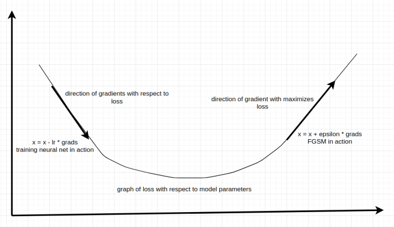
Gradient descent is an optimization strategy employed in machine learning to minimize a loss function. The objective is to fine-tune model parameters in a way that decreases the value of the loss function, thereby improving the model’s performance.

Given a loss function \(J(\theta) \), where \(\theta \) represents the model’s parameters, the gradient descent update step can be expressed as:

Here:

• \(\alpha \) is the learning rate, determining the step size of the update.
• \(\nabla_\theta J(\theta) \) is the gradient of the loss function with respect to the parameters \(\theta \).

The negative sign before \(\alpha \) ensures that we move in the direction opposite to the gradient. This enables us to descend along the slope of the loss function and converge towards a minimum.

Fast Gradient Sign Method (FGSM): Maximizing Loss

Now, let’s delve into the Fast Gradient Sign Method (FGSM).

Fast Gradient Sign Method is a white-box attack that computes an adversarial image by adding a pixel-wise perturbation of magnitude in the direction of gradient with respect to the loss function.

For a non-targeted attack, the FGSM computes the adversarial image \(x_{adv} \) as follows:

We maximize

subject to

In case of targeted attack, direction is negative gradient with respect to the target class:

where \(x\) is clean input image, \(x_{adv}\) is corresponding adversarial image, \(J\) is classification loss, \(y_{true}\) is actual label, \(y_{target}\) is target label and \(\epsilon\) is \(L_\infty\) budget.

The core concept is to add a perturbation scaled by \(\epsilon \) in the direction of the gradient of the loss function with respect to the input \(x \). This perturbation maximizes the loss and consequently deceives the model’s prediction.

The model’s weights remain constant and the gradient is computed only with respect to the input and not the model’s weights. The size of the perturbation is controlled using \(\epsilon \). The sign gives the direction of the gradient. FGSM is fast since it is easy to compute the contribution of each pixel to the loss function by finding gradients and adding a perturbation accordingly to maximize the loss. However, this simplicity also means that may not always produce the most optimized adversarial example that is close to the benign image, and can be more easily defended against compared to iterative methods.

Hypothesis of FGSM Exploiting Linearity

The fast gradient sign method (FGSM) was introduced by Goodfellow et al. (2015). They hypothesize that neural networks use linear techniques for optimization and therefore are vulnerable to linear attacks. FGSM takes advantage of the gradient information, which represents the linear approximation of the loss function around a specific input point. This process of leveraging the linearity of the gradient to influence the model’s decision causes it to misclassify the adversarial example.

However, it’s important to note that while linearity plays a significant role, the vulnerability of neural networks to adversarial attacks also involves non-linear aspects that further contribute to their susceptibility. Non-linear activation functions like ReLU, sigmoid, or tanh introduce non-linearity into computation. These non-linearities can be exploited by perturbing the inputs in ways that trigger specific activations, and influence the decision making process of the model.

Summarizing FGSM

Given a trained deep learning model and an input image, the attack can be summarized in the following steps:

1. Forward pass: Pass the input image through the model and compute the loss based on the predicted class.
2. Gradient computation: Compute the gradients of the loss with respect to the input image by backpropagating through the model.
3. Perturbation calculation: Perturb the input image by adding the sign of the computed gradients (or the sign of the gradient multiplied by epsilon) to the original image.
4. Adversarial example generation: Generate the adversarial example by adding the perturbation to the original image.
5. Adversarial classification: Feed the adversarial example into the model and observe the misclassification or the desired target label.

Getting Hands-On with FGSM

In extension to a previous post where I fine-tuned a ResNet-50 model pretrained on ImageNet for CIFAR-10, I achieved an accuracy of 92.34% on the test set. I will be using my previous project as base and build the attack on the fine-tuned model. I’ve only added a few utility plotting functions and ofcourse, added the FGSM code to generate adversarial examples.

The below FGSM code is simple to understand if one follows my summary above.

def fgsm_attack(model, criterion, images, labels, device, epsilon):
    images.requires_grad_(True)
    outputs = model(images)
    loss = criterion(outputs, labels).to(device)
    model.zero_grad()
    loss.backward()

    gradient = images.grad.data
    perturbations = epsilon * torch.sign(gradient)
    adversarial_images = images + perturbations
    adversarial_images = torch.clamp(adversarial_images, 0, 1)

    return adversarial_images, perturbations

Testing Robustness of ResNet-50 against FGSM

The code below tests the accuracy of the fine-tuned ResNet-50 model against adversarial examples generated by FGSM.

• Adversarial Accuracy is measured as the percentage of adversarial images that are correctly classified by the model.
  This is a measure of the robustness of the model against the attack.
• Attack Success Rate is measured as the percentage of adversarial images that are misclassified, among benign inputs that are correctly classified by the model.
  This is a measure of robustness of the attack against the model.

def test_adversarial(model, testloader, criterion, device, epsilon):
    adversarial_correct = 0
    attack_success = 0
    total = 0

    model.eval()

    for images, labels in testloader:
        images, labels = images.to(device), labels.to(device)

        adversarial_images, _ = fgsm_attack(model, criterion, images, labels, device, epsilon)

        adversarial_outputs = model(adversarial_images)

        _, adversarial_predicted = torch.max(adversarial_outputs.data, 1)

        adversarial_correct += (adversarial_predicted == labels).sum().item()
        attack_success += (adversarial_predicted != labels).sum().item()
        total += labels.size(0)

    adversarial_accuracy = 100.0 * adversarial_correct / total
    attack_success_rate = 100.0 * attack_success / total
    print(f'Epsilon = {epsilon}:')
    print(f'Adversarial Accuracy: {adversarial_accuracy:.2f}%')
    print(f'Attack Success Rate: {attack_success_rate:.2f}%')
    print('------------------------------------------------------')
    return adversarial_accuracy, attack_success_rate

Flow of Code

The seed is set for reproducibility. The dataset and model are loaded. The model’s first convolutional layer is modified to suit CIFAR-10 dataset such that there is lesser loss of spatial information. The fully connected layer is also modified to suit CIFAR-10’s 10 classes.

The loss function is CrossEntropy, optimizer is Stochastic Gradient Descent with a learning rate of 0.001, momentum of 0.9, epoch=. The size of perturbation is set to 0.3.

First the model is trained and the accuracy is calculated on the clean test set. Then the best model saved is loaded and tested against the adversarial examples. A list of epsilon values can be used to compare how the size of perturbation can affect the results. Finally, the adversarial examples are visualized.

def main(train_model, epsilon_list):

    # Set random seeds for reproducibility
    random.seed(42)
    np.random.seed(42)
    torch.manual_seed(42)

    # Load the dataset
    num_classes = 10
    batch_size = 64
    trainset, trainloader, testset, testloader, classes = load_dataset(batch_size)

    # Load the pre-trained model
    model = models.resnet50(pretrained=True)
    # Modify conv1 to suit CIFAR-10
    model.conv1 = nn.Conv2d(3, 64, kernel_size=3, stride=1, padding=1, bias=False)
    # Modify the final fully connected layer according to the number of classes
    num_features = model.fc.in_features
    model.fc = nn.Linear(num_features, num_classes)
    # Move the model to GPU if available
    device = torch.device('cuda' if torch.cuda.is_available() else 'cpu')
    model = model.to(device)

    # Set hyperparameters
    criterion = nn.CrossEntropyLoss()
    optimizer = optim.SGD(model.parameters(), lr=0.001, momentum=0.9)
    num_epochs = 60
    epsilon = 0.3
    epsilon_values = [0.01, 0.03, 0.07, 0.1, 0.3, 0.5]

    if train_model:
      print("Training the model...")
      # Train the model
      model, train_losses, train_accuracies, test_losses, test_accuracies = train_epochs(
          model, trainloader, testloader, criterion, optimizer, device, num_epochs)

      # Plot the loss and accuracy curves
      plot_loss(train_losses, test_losses)
      plot_accuracy(train_accuracies, test_accuracies)
      # Plot and save an example image
      plot_image(testset, model, classes, device)
      # Visualize some adversarial examples
      print("Generating Visualization Plot")
      plot_adv_images(testset, model, criterion, classes, device, epsilon)  
    else:
      # Load the best model
      best_model = models.resnet50(pretrained=True)
      # Modify conv1 to suit CIFAR-10
      best_model.conv1 = nn.Conv2d(3, 64, kernel_size=3, stride=1, padding=1, bias=False)
      best_model.fc = nn.Linear(num_features, num_classes)
      # Load checkpoints
      checkpoint = torch.load('best_model.pth')
      best_model.load_state_dict(checkpoint['model_state_dict'])
      epoch = checkpoint['epoch']
      test_accuracy = checkpoint['test_accuracy']
      best_model = best_model.to(device)
      print("Best Trained Model Loaded!")
      print(f"Checkpoint at Epoch {epoch+1} with accuracy of {test_accuracy}%")

      # Test the best model on adversarial examples
      if epsilon_list:
        # Evaluate adversarial attacks for each epsilon value
        adversarial_accuracies = []
        attack_success_rates = []
        print("Testing with clean data again to compare with checkpoint accuracy...")
        _, clean_test_accuracy = test(best_model, testloader, criterion, device)
        print(f"Clean Adv Accuracy: {clean_test_accuracy:.2f}%\nClean Attack Success Rate: {100-clean_test_accuracy:.2f}%")
        if(clean_test_accuracy==test_accuracy):
          print("Matches with the Checkpoint Accuracy!")
        print('-----------------------------')
        print("Testing with adversarial examples...")
        for epsilon in epsilon_values:
          adversarial_accuracy, attack_success_rate = test_adversarial(best_model, testloader, criterion, device, epsilon)
          adversarial_accuracies.append(adversarial_accuracy)
          attack_success_rates.append(attack_success_rate)
        epsilon_compare(epsilon_values, adversarial_accuracies, attack_success_rates)
      else:
        clean_adversarial_accuracy, clean_attack_success_rate = test_adversarial(best_model, testloader, criterion, device, epsilon)
        print(f"Clean Adv Accuracy: {clean_adversarial_accuracy}\nClean Attack Success Rate: {clean_attack_success_rate}")
        # Visualize some adversarial examples
        print("Generating Visualization Plot")
        plot_adv_images(testset, best_model, criterion, classes, device, epsilon)

The Main Function

The main() function is the entry point for the program.

If train_model is set to True, the function trains the model. The function first trains the model for num_epochs epochs. After each epoch, the function plots the loss and accuracy curves. The function then plots and saves an example image.

• With train_model set to True, “epsilon_list” should be False to get the plots of adversarial examples and avoid any errors.

Effect of Perturbation Size

If train_model is set to False, the function loads the best model from a checkpoint.

• If the “episilon_list” is set to False, the function visualizes some adversarial examples.
• If the “episilon_list” is set to True, the function uses a list of “epsilon_values” and runs the test_adversarial() function for all the values and then compares them.

if __name__ == '__main__':
    main(train_model=True, epsilon_list=False)
    main(train_model=False, epsilon_list=True)

Results

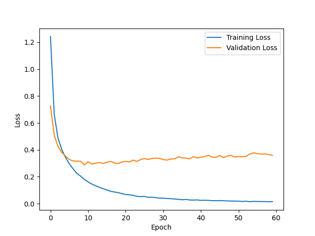
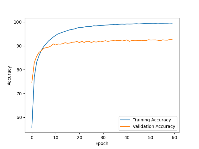
• After training the model for 60 epochs, it achieved a clean test accuracy of 92.63%.
• The model is slightly overfitting.

Let’s look at some randomly picked clean test data and their respective perturbation and adversarial example.

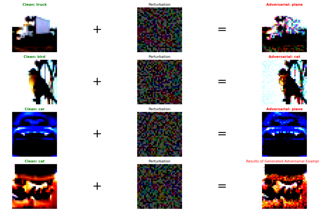
The adversarial images look pixelated at just 0.3 perturbation size as CIFAR-10’s input size is 32×32. As observed from the above results, all the randomly selected images are misclassified.

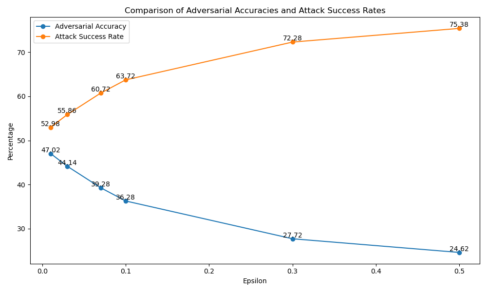
• The model was then tested with adversarial examples generated using different epsilon values. With an epsilon of 0.01, the adversarial accuracy dropped to 47.02%, indicating successful attacks on the model.
• As the epsilon value increased, the adversarial accuracy decreased further, reaching 24.62% at an epsilon of 0.5.
• The attack success rate increased with higher epsilon values, ranging from 52.98% at epsilon 0.01 to 75.38% at epsilon 0.5.

Discussion

During my Master’s thesis on the same topic, I often pondered whether to focus only on correctly classified images during the testing of adversarial images or to use the full dataset. In the “test_adversarial” function, I would switch between using the code we used for this experiment and the below code that uses a filtered dataset approach that only considers images were correctly classified by the model, instead of considering a benign image that was misclassified to be a successfully generated adversarial image.

def test_adversarial(model, testloader, criterion, device, epsilon):
    adversarial_correct = 0
    attack_success = 0
    total = 0

    model.eval()

    for images, labels in testloader:
        images, labels = images.to(device), labels.to(device)

        adversarial_images, _ = fgsm_attack(model, criterion, images, labels, device, epsilon)

        adversarial_outputs = model(adversarial_images)

        _, adversarial_predicted = torch.max(adversarial_outputs.data, 1)

        # Update statistics only for correctly classified clean images
        original_outputs = model(images)
        _, original_predicted = torch.max(original_outputs.data, 1)
        correct_mask = (original_predicted == labels)

        adversarial_correct += (adversarial_predicted[correct_mask] == labels[correct_mask]).sum().item()
        attack_success += (adversarial_predicted[correct_mask] != labels[correct_mask]).sum().item()
        total += correct_mask.sum().item()

    adversarial_accuracy = 100.0 * adversarial_correct / total
    attack_success_rate = 100.0 * attack_success / total
    print(f'Epsilon = {epsilon}:')
    print(f'Adversarial Accuracy: {adversarial_accuracy:.2f}%')
    print(f'Attack Success Rate: {attack_success_rate:.2f}%')
    print('------------------------------------------------------')
    return adversarial_accuracy, attack_success_rate

With this modification, the total count now accurately reflects the number of correctly classified images in the adversarial set, and the adversarial_correct count only considers cases where the adversarial image was correctly classified after the attack, regardless of whether the original prediction was correct.

Here are some considerations for both approaches:

Filtered Dataset Approach (Considering Only Correctly Classified Images):

Pros:

1. Reflects the true adversarial impact: By focusing only on correctly classified images, you are measuring the effectiveness of the attack on images that the model is confident in its predictions.
2. May provide more meaningful results: Excludes misclassified examples that might be outliers or not representative of the model’s typical performance.

Cons:

1. Variability: Different researchers might have different models with varying levels of performance, which could lead to varying filtered dataset sizes.
2. Difficulty in comparisons: It might be harder to directly compare results across studies if different filtering strategies are used, potentially making it less standardized.

Full Dataset Approach (Including All Images):

Pros:

1. Standardization: Using the full dataset size ensures consistency across different researchers and models, allowing for easier comparisons.
2. Reflects overall model performance: Provides a comprehensive view of how the model performs on the entire dataset, including correctly and misclassified images.

Cons:

1. Diluted adversarial impact: Including misclassified images in the calculation of attack success rate might obscure the true effectiveness of the adversarial attack.
2. Less discriminative: Misclassified images could be treated as adversarial even if the model’s misclassification is not due to the adversarial perturbation.

Ultimately, the choice between these approaches should be guided by the goals of your research and the insights you want to convey.

If your primary focus is to demonstrate the effectiveness of adversarial attacks on correctly classified images (which is a valid and interesting research question), then using the filtered dataset approach might be appropriate.

On the other hand, if you aim to provide a standardized and easily comparable measure of adversarial impact, the full dataset approach that we used in this experiment could be more suitable.

Conclusion

In conclusion, the Fast Gradient Sign Method (FGSM) is an efficient adversarial attack technique that leverages gradient information to create perturbations. FGSM’s simplicity allows for fast computation of perturbation contributions, but it may not always produce the most optimized adversarial examples. When applied to a fine-tuned ResNet-50 model with an accuracy of 92.63% on clean test set, FGSM demonstrated a drop in accuracy to 24.62% on adversarial examples at an epsilon value of 0.5, indicating successful attacks.

Selecting an appropriate epsilon value, which controls the perturbation size, is crucial, as higher epsilon values increase attack success rates but may also increase the detectability of the adversarial examples. The FGSM technique underscores the vulnerability of deep learning models and the importance of developing robust defense mechanisms in Adversarial Machine Learning.

In the next part of this series, we’ll be focusing on targeted attacks where we craft perturbations such that the model misclassifies to the specified target class.