Summary of AlexNet

Title: ImageNet Classification with Deep Convolutional Neural Networks (2012)
Authors: Alex Krizhevsky, Ilya Sutskever, Geoffrey E. Hinton
Point of the Paper: “GPU memory enables training large networks on large image datasets.”
At a time when human performance was achieved on relatively small image datasets like MNIST and CIFAR-10, computer vision researchers were eager to achieve the same with large, high-resolution image datasets. Although datasets such as ImageNet provided large and real-world data, simple convolution neural networks (CNN) did not perform well on such high-resolution datasets. Innovative trials were limited by computational resources. AlexNet solved these problems by introducing deep CNN that achieved the state-of-the-art in the ImageNet LSVRC-2010 contest, and GPU parallelization.
Need for Large Datasets and Large Networks
To learn about thousands of objects from millions of images, we need a model with a large learning capacity.
Large datasets provide better data distribution with a more accurate mean to help generalize to the real world input data that may not belong to the same training set distribution. AlexNet was strained on ImageNet, which consists of roughly 1 million high-resolution images for the 1000 category subset used in the ILSVRC contest. While large datasets come in handy to afford simple models to classify outliers better, large image datasets need robust models to learn as much information as possible to generalize better. Therefore, the authors aimed to build a model with a large learning capacity. Statistically, pixels are correlated by the distance between them. CNNs try to exploit this correlation to learn. Instead of using a simple feed forward network, the authors chose to go deeper by varying the width (adding nodes to learn features) and depth (adding layers) of the CNN. And so, AlexNet took birth to beat the previous state-of-the-art.
Architecture of AlexNet
The CNN consists of 8 layers. The first 5 layers are convolutional layers and the last three are fully connected layers. The last fully connected layer is forwarded to a 1000 way softmax to get the class probabilities.

Faster Learning with ReLU and GPUs
ReLU vs Tanh
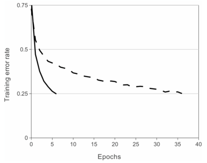
Deep convolutional neural networks with ReLUs train several times faster than their equivalents with tanh units.

While the modern activation functions are Leaky/ReLU, tanh, and sigmoid were the conventional nonlinear activation functions to train neural networks. Although nonlinear activation functions are preferred as most problems require a neural network to produce a nonlinear decision boundary, saturating nonlinear functions such as sigmoid and tanh not only limit the learning of the model at the boundaries but are also computationally expensive. The backpropagation during training in ReLU is computationally inexpensive since it uses a simple max function between input and zero instead of exponential calculation, and the derivative is either 0 or 1. The ReLU function does not saturate at extreme values and prevents zero slopes, hence preventing vanishing gradient problem as seen in sigmoidal or tanh functions. The experiment to compare the performance between ReLU and TanH on CIFAR-10 showed that ReLU accelerates gradient descent optimization, allowing to train faster than the tanh neurons.

Multiple GPUs
At the time of writing this post, a college student could be equipped with an RTX 3090 with 10496 cores and 24GB of memory in a single GPU to perform computer vision tasks where as Alexnet was trained on a GTX 580 with 512 cores and 3GB memory. The challenge of training a large dataset on a deep CNN, with the available GPU was addressed by GPU parallelization. The 1.2 million training examples and the model had to be spread across two GTX 580 GPUs. This parallelization scheme reduced the top-1 and top-5 error rates by 1.7% and 1.2% respectively, as compared to training on one GPU.
Local Response Normalization (LRN)
A well known effect in neuroscience is that a strongly active neuron will tend to suppress the neighbouring neurons. The idea of local response normalization is to encourage inhibition of the neurons nearby. A local maxima creates a desirable contrast in that particular area of the feature map, therefore capturing necessary information only. Since ReLU does not require the input to be normalized, the output of ReLU can be large. LRN recognizes the high activation neurons and normalizes the local neighbourhood of the exited neuron and also dampens equally high activation neurons, thus highlighting only the peaks. The enhancement of peaks and normalization of flat, strong responses provides desirable stimuli for the neural network. It reduces the top-1 and top-5 error rates by 1.4% and 1.2% respectively. On CIFAR-10, a four layer CNN achieved a 13% test error rate without normalization and 11% with normalization.
Overlapping Pooling
Pooling is used to downsample an input and summarize the features of a group of neurons of a filter. It also increases speed of computation by reducing the parameters to learn. A filter size is greater than the stride leads to overlap. Pooling reduces the number of features and addresses the problem of overfitting. Alexnet used a stride of 2 and filter size of 3 as hyperparameters for max pooling. This reduced the top-1 and top-5 error rates by 0.4% and 0.3% respectively.
Reducing Overfitting
Alexnet’s large network has 60 million parameters. The VC dimension (Vapnik-Chervonenkis) of a neural network is approximately equal to the number of parameters in the model. To train a model, the relation between the VC dimension of a neural network and number of examples is linear. Therefore, number of examples should linearly grow with the network’s hypothesis; which means we need 60 million examples to train Alexnet. Alexnet was able perform well despite lack of training examples because they used different techniques such as data augmentation and dropout.
Data Augmentation
To reduce overfitting by increasing the number of examples, data augmentation was used. The first type of data augmentation consisted of image translations and horizontal reflections. This increased the size of training set by a factor of 2048. At test time, four corner patches and centre patch of 224×224 were extracted along with their horizontal reflections. The second type of augmentation consisted of altering the pixel intensities by performing principle component analysis (PCA) on the RGB channels in training images. The principal components of each channel were extracted and multiples of the principal components were added to the pixel. The labels of the images are not altered by this change in intensities. This reduced the top-1 error rate by over 1%.
Dropout
Dropout randomly sets neurons to zero at each update of the training phase. By nullifying the nerons, it disables any previous batch of training examples to influence the learning and reduce redundant learning which helps the model to learn robust features and generalize better. Although this is the only section where authors do not mention quantitative results like error rate, it was mentioned that dropout helped reduce overfitting but doubles the number of iterations required to converge.
Details of Learning
The most interesting part of the details apart from stochastic gradient descent as optimization, batch size of 128, momentum of 0.9, and weight decay of 0.0005 is that they initialized the weights in each layer from a zero-mean Gaussian distribution with standard deviation 0.01. The parameters will have an average value close to zero and standard deviation of some small number. When the model is first learning, the result will be zero mean. If input is zero-mean, then the expectation of value of that unit over training set would also be zero. Since ReLU is being used, zero-mean inputs will output zero which will eventually disable learning. To counter this effect of ReLU, they use bias. Other hyperparameters include initializing learning rate of 0.01 and divide the learning rate by 10 when validation error rate stopped improving. Setting learning rate is crucial when using ReLU because it outputs zero too soon. Modern networks use Leaky ReLU so that the network eventually learning even if the value is in the negative range. The network was trained for 90 iterations which took five to six days on two NVIDIA GTX 580 3GB GPUs.
Results
The best results in the ILSVRC-2010 were 47.1% and 28.2% top-1 and top-5 error rates respectively. Alexnet was able to outperform this result with a 37.5% top-1 and 17.0% top-5 error rate. Alexnet won the 2012 contest with 36.7% top-1 and 15.3% top-5 error rates compared to the second place winners top-5 error rate of 25.2%.
Conclusion
Students don’t need RTX 3090s to build great models.


February 26, 2022 @ 4:34 AM
Really insightful! Thanks a lot