Traffic Sign Detection with Faster R-CNN
Autonomous vehicles that are capable of navigating without human inputs are heavily dependent on computer vision tasks such as object detection. Many object detection algorithms such as YOLO, Faster R-CNN, SSD, have been proposed to detect and recognize the traffic signs.
In this blog, Faster R-CNN will be used for the detection of German traffic signs (GTSDB dataset) with reference to Torchvision’s object detection finetuning tutorial.
R-CNN
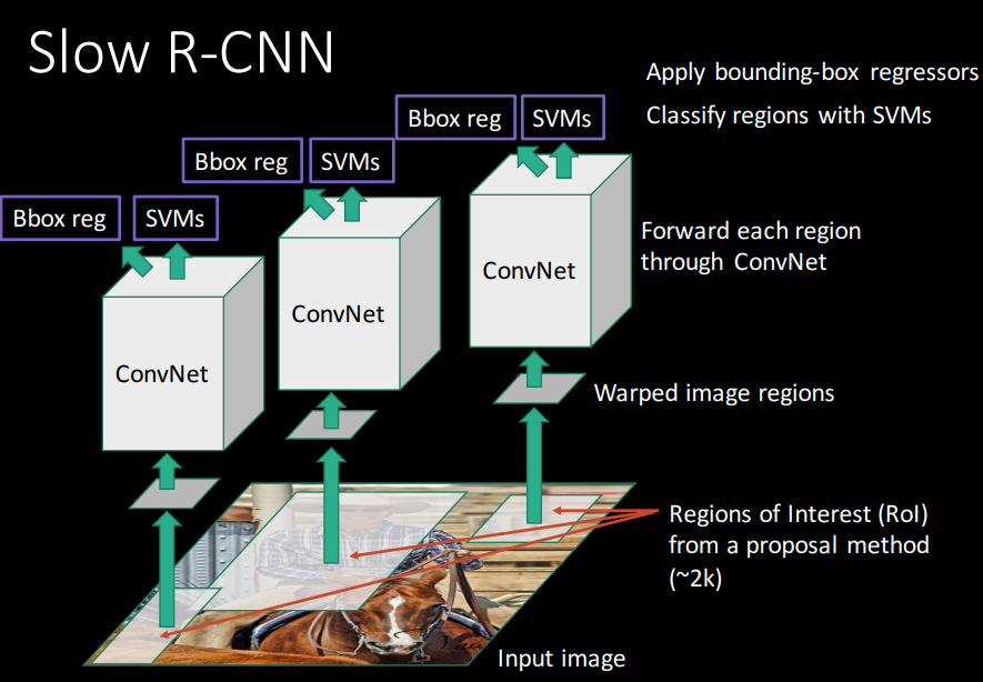
The intuition of region based CNN’s is to use selective search to extract 2000 regions from an image. In selective search algorithm, sub-segmentation is performed to generate candidate regions and similar regions are grouped into a single entity to be used as a candidate region proposal. These candidate regions proposals or region of interest (RoI) are passed through the CNN to output a feature map for each region. These regions are classified by using SVMs. Finally, bounding box regression is used to predict the bounding box coordinates for each region. Slides by Ross Girshick explain this well.
Faster R-CNN
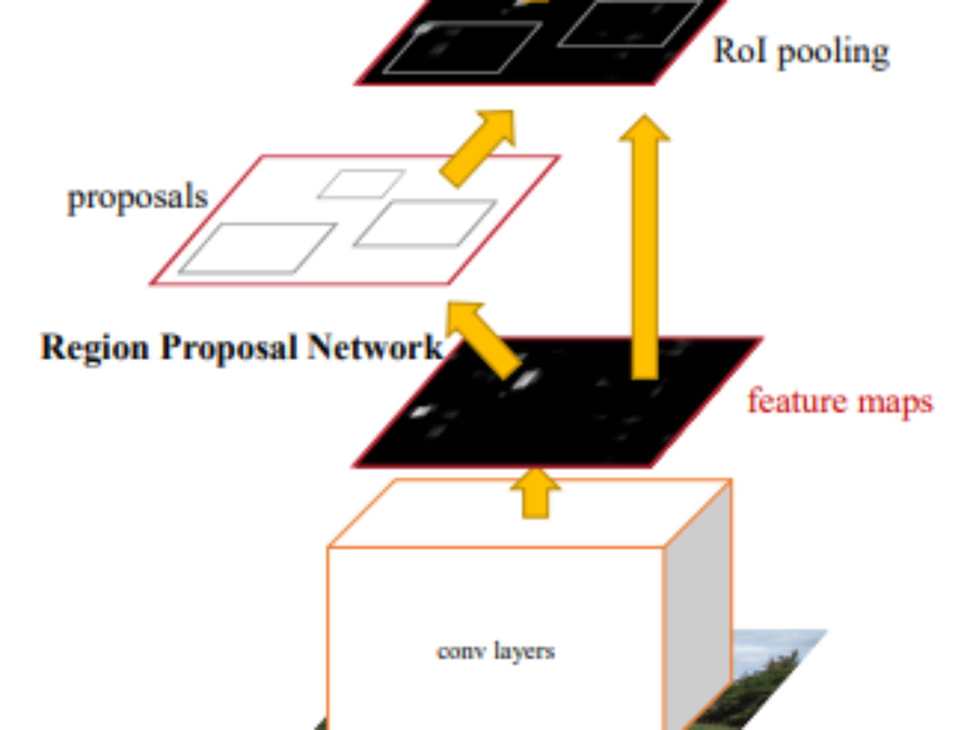
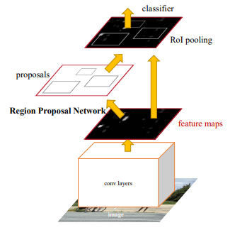
Instead of using selective search for generating RoI, Faster R-CNN uses a separate network called Region Proposal Network (RPN) to generate region proposals from feature maps outputted by CNN. RPN uses a sliding window over these feature maps and generates anchor boxes of different dimensions. These anchor boxes are used by the RPN to predict the existence of an object and a bounding box that tightly fits the object. The predicted regions are reshaped to the same size by using a RoI pooling layer. Finally, these anchor’s feature maps are passed to a fully connected layer that classifies the object and predicts the bounding box coordinates for the objects.
Getting Started
Feel free to follow the Jupyter notebook in my Github along with this blog post to check the output of the code.
German Traffic Sign Detection Benchmark (GTSDB) dataset is used.
Download the dataset!
COCO Evaluation metrics and some transform functions were used in this code. The Torchvision’s Git Repository provides an API for COCO evaluation, transforms and other useful stuff used in object detection. These files are required to be placed in the root directory of the project: utils.py, engine.py, coco_eval.py, coco_utils.py, transforms.py.
Note: I had some conflicts while importing these files. For example, utils.py. They probably won’t work out of the box. I’ve also made a few simple changes to return evaluation metrics while training, you could download the files I used from my Git Repository.
Organizing the GTSDB Dataset
Unzipping the dataset zip, there are class folders with respective images and .ppm files. There is also the annotation file named as gt.txt
Copy all the .ppm files from the TrainIJCNN2013 folder to a directory named “train/images”.
Importing Libraries
Install “pycocotools” along with other required libraries.
import os
import numpy as np
import pandas as pd
from glob import glob
import cv2
import torch
from torch.utils import data
from PIL import Image
import torchvision
from torchvision import transforms
import matplotlib.pyplot as plt
Handling Image Data and Annotations
The “gt.txt” file is used here to create a dictionary with the image names as key and annotations + class ID as value. If an image contains multiple objects then the coordinates along with the class is stored as list of lists in the same dictionary’s key.
txt = np.genfromtxt('train/gt.txt',delimiter =';', dtype= None,encoding=None)

#Creating a dictionary with image names as key and annotations as value
dic ={}
for i in range (0,len(txt)):
    #Image name is first element of annotation file
    img_name = txt[i][0]
    # 4 Coordinates
    target = [txt[i][1],txt[i][2],txt[i][3],txt[i][4],txt[i][5]]
    #Last element is the class number
    clas = txt[i][-1]
    #If multiple objects, store coordinates and classes as list of lists
    if(img_name in dic):
        dic[img_name].append(target)
    else:
        dic[img_name] = [target]
print(dic['00001.ppm'])
print("Number of Images: " + str(len(dic)))
Data Distribution
Let’s plot the data distribution.
#Data Distribution

cls_lst = {}

for i in dic:
    for j in dic[i][:]:
        #print(len(dic[i]))
        for k in range(len(dic[i])):
            clss = dic[i][:][k][-1]
            if clss in cls_lst:
                cls_lst[clss] += 1
            else:
                cls_lst[clss] = 1

print(cls_lst)

xx = []
yy = []
for i in cls_lst:
    xx.append(str(i))
    yy.append(cls_lst[i])

x_pos = [i for i, _ in enumerate(xx)]

plt.bar(x_pos, yy, color='green')
plt.xlabel("Class Number")
plt.ylabel("Number of Examples")
plt.title("GTSDB")
#plt.figure(figsize=(30,30))
plt.xticks(x_pos, xx)

plt.show()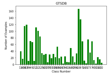
From the plot, it is evident that the distribution of data is not equal. Some classes have insufficient examples.
Data Cleaning
The images without annotations can’t be used while training the model. Therefore, the images which have annotations should only be used. These images are copied to a new folder.
#Copy only files that are annotated in the gt.txt to imagesf
import shutil

pt = glob('./train/images/*.ppm')

len(pt)
#Copying into new directory
for i in range(len(dic)):
    ofile = r'./train/images/{}'.format(list(dic)[i])
    target = r'./train/imagesf/{}'.format(list(dic)[i])
    shutil.copyfile(ofile, target)
#Check if len(dic) == number of images in folder
print(len(glob('./train/imagesf/*.ppm')))
len(dic)
The directory structure should look like this:
- train
- images
- *.ppm
- imagesf
- *.ppm
- gt.txt
- images
- utils.py
- engine.py
- transforms.py
- coco_eval.py
- coco_utils.py
Defining Custom PyTorch Dataset Class
The below code fetches all the required data from the dataset while reading.
class myDataset(torch.utils.data.Dataset):
    def __init__(self, root, transforms=None):
        self.root = root
        self.transforms = transforms
        # load all image files, sorting them to ensure that they are aligned
        self.imgs = list(sorted(os.listdir(os.path.join(root, "imagesf"))))

    def __getitem__(self, idx):
        # Load image path
        img_path = os.path.join(self.root, "imagesf", self.imgs[idx])
        #Load image as PIL
        img = Image.open(img_path).convert("RGB")
        # Get objects in the image
        objects = dic[self.imgs[idx]]
        # Get bounding box coordinates for each object in image
        boxes = []
        labels = []
        for obj in objects:
            #print(idx, obj[-1], self.imgs)
            name = obj[-1]
            labels.append(np.int(name))
            #Get bounding box coordinates
            xmin = np.float(obj[0])
            ymin = np.float(obj[1])
            xmax = np.float(obj[2])
            ymax = np.float(obj[3])
            boxes.append([xmin, ymin, xmax, ymax])

        boxes = torch.as_tensor(boxes, dtype=torch.float32)
        labels = torch.as_tensor(labels, dtype=torch.int64)

        image_id = torch.tensor([idx])
        area = (boxes[:, 3] - boxes[:, 1]) * (boxes[:, 2] - boxes[:, 0])
        # suppose all instances are not crowd
        iscrowd = torch.zeros((len(objects),), dtype=torch.int64)

        target = {}
        target["boxes"] = boxes
        target["labels"] = labels
        target["image_id"] = image_id
        target["area"] = area
        target["iscrowd"] = iscrowd

        if self.transforms is not None:
            # Note that target (including bbox) is also transformed\enhanced here, which is different from transforms from torchvision import
            # Https://github.com/pytorch/vision/tree/master/references/detectionOfTransforms.pyThere are examples of target transformations when RandomHorizontalFlip
            img, target = self.transforms(img, target)

        return img, target

    def __len__(self):
        return len(self.imgs)
Here’s what happens in the myDataset (torch.utils.data.Dataset) class:
- Initialize all the required variables: Root directory of images (path), transforms (boolean), imgs (images dir in root).
- According to PyTorch’s documentation, the Dataset class should implement getitem and len methods. So we declare them.
- In the getitem method, for each image we take the annotations and labels as input from the dictionary we created before. We store them in ‘objects’ variable.
- A ‘targets’ dictionary is then initialized to pass all the data to the model while training.
- ‘area’ declared for the evaluation metrics of COCO API. It separates the metric scores between small, medium and large boxes.
- ‘iscrowd=True’ will ignore all instances with numerous objects in one image.
- ‘image_id’ is an image identifier. It is unique between all images in the dataset and is used during evaluation.
- ‘transforms=True’ will call the transforms function to apply transformations.
- len method returns the size of the Dataset.
Refer to the PyTorch’s Object Detection Tutorial
Data Augmentation using PyTorch’s Tranforms
The images are enhanced before being passed to the network. The images are transformed using the functions defined in the “transforms.py” file in pytorch/vision.
The difference between original and transformed images are shown in the results.
import utilss
import transforms as T
from engine import train_one_epoch, evaluate
# utils, transforms, engine were just downloadedUtils.py,transforms.py,engine.py

def get_transform(train):
    transforms = []
    # converts the image, a PIL image, into a PyTorch Tensor
    transforms.append(T.ToTensor())
    if train:
        # during training, randomly flip the training images
        # and ground-truth for data augmentation
        # 50% chance of flipping horizontally
        transforms.append(T.RandomHorizontalFlip(0.5))

    return T.Compose(transforms)
Defining the Model and Loading Data:
- The number of classes is 44 since there are 43 classes + background
- Then declare train and test dataset by calling the myDataset class which was defined earlier.
- Split the dataset into two 4:1 Train to Test approximately.
- Use PyTorch’s DataLoader to load data.
- Define the model. Faster RCNN with a pretrained ResNet50 backbone network is used to finetune according to our dataset.
- Since I had 4 RTX 2080 GPU’s available, I was able to train on all GPUs parallely.
from engine import train_one_epoch, evaluate
import utilss
import torch.nn as nn
os.environ['TORCH_HOME'] = './'

root = r'./train'

# Train on the GPU if available else CPU.
device = torch.device('cuda') if torch.cuda.is_available() else torch.device('cpu')

# 44 classes = 43 + background
num_classes = 44
#Send the data to the myDataset class (Apply transformations, Get bbox, labels, objects)
dataset = myDataset(root, get_transform(train=True))
dataset_test = myDataset(root, get_transform(train=False))

# split the dataset in train and test set
# My dataset has 506 images, almost training validation 4:1
indices = torch.randperm(len(dataset)).tolist()
dataset = torch.utils.data.Subset(dataset, indices[:-100])
dataset_test = torch.utils.data.Subset(dataset_test, indices[-100:])

# define training and validation data loaders
#collate_fn returns tuples of images and image annotations for every iteration.
data_loader = torch.utils.data.DataLoader(
    dataset, batch_size=2, shuffle=True, # num_workers=4,
    collate_fn=utilss.collate_fn)

data_loader_test = torch.utils.data.DataLoader(
    dataset_test, batch_size=2, shuffle=False, # num_workers=4,
    collate_fn=utilss.collate_fn)

# Define model
model = torchvision.models.detection.fasterrcnn_resnet50_fpn(pretrained=False, progress=True, num_classes=num_classes, pretrained_backbone=True)
# OR model = get_object_detection_model(num_classes)
#model = torch.load('./train150.pkl')

#Use specific GPUs:
model = nn.DataParallel(model, device_ids=[0,1,2,3]) #Remove this line if not necessary.

# Move the model to device
model.to(device)

print("Model loaded")
Training the Model:
Here’s what happens in the code below:
- Defining all the parameters required for training. (Using SGD as optimizer, Cosine Annealing/Decreasing Warm Restarts as learning rate scheduler which decreases the initial learning rate set in a cosine manner until a restart; the lr is set back to the initial lr and the cycle repeats, number of epochs = 1000)
- Declaring all the variable to be retrieved from the COCO Evaluation metrics.
- We start train them model and evaluate the performance on test set.
Here, train_one_epoch function in engine.py is used to do the training. The train_one_epoch function returns metric_logger object which we store in ‘metrics’. We use the metric_logger’s attributes (losses) to append into their respective variables.
Then, the evaluate method in CocoEvaluator() in coco_eval.py returns a coco_eval object which is stored in ‘ _ ‘. We use this coco_eval object to retrieve the stats attribute from pycocotools’ library’s summarize(). We append them to all the stat variables to later plot them after training.
from engine import train_one_epoch, evaluate
import utilss
from IPython.display import clear_output
import pickle


# Constructing the optimizer
params = [p for p in model.parameters() if p.requires_grad]

# SGD
optimizer = torch.optim.SGD(params, lr=0.0005,
                            momentum=0.9, weight_decay=0.0005)

# Learning Rate Scheduler
lr_scheduler = torch.optim.lr_scheduler.CosineAnnealingWarmRestarts(optimizer, T_0=1, T_mult=2)

# Training for no. of Epochs
num_epochs = 1000


losses = []
loss_box_reg = []
loss_rpn_box_reg = []
loss_classifier = []
loss_objectness = []

stat0 = []
stat1 = []
stat2 = []
stat3 = []
stat4 = []
stat5 = []
stat6 = []
stat7 = []
stat8 = []
stat9 = []
stat10 = []
stat11 = []


for epoch in range(num_epochs):
    # Engine.py's train_one_epoch function takes both images and targets. to(device)
    # Metrics (metric_logger) was returned by train_one_epoch() in engine.py to get losses
    metrics = train_one_epoch(model, optimizer, data_loader, device, epoch, print_freq=50)
    losses.append(float(str(metrics.meters['loss']).split(" ")[0]))
    loss_box_reg.append(float(str(metrics.meters['loss_box_reg']).split(" ")[0]))
    loss_rpn_box_reg.append(float(str(metrics.meters['loss_rpn_box_reg']).split(" ")[0]))
    loss_classifier.append(float(str(metrics.meters['loss_classifier']).split(" ")[0]))
    loss_objectness.append(float(str(metrics.meters['loss_objectness']).split(" ")[0]))

    # Update the learning rate
    lr_scheduler.step()

    # Evaluate on the test dataset
    # _ gives coco_evaL obj from coco_eval.py from CocoEvaluator()
    _, metric_logger = evaluate(model, data_loader_test, device=device)
    #Stat object is from pycocotools' self.stats in summarize()
    #https://github.com/cocodataset/cocoapi/blob/master/PythonAPI/pycocotools/cocoeval.py
    stat = _.coco_eval['bbox'].stats

    #Append all stats
    stat0.append(stat[0])
    stat1.append(stat[1])
    stat2.append(stat[2])
    stat3.append(stat[3])
    stat4.append(stat[4])
    stat5.append(stat[5])
    stat6.append(stat[6])
    stat7.append(stat[7])
    stat8.append(stat[8])
    stat9.append(stat[9])
    stat10.append(stat[10])
    stat11.append(stat[11])


    print('')
    print('==================================================')
    print('')

print("Done!")
Evaluation
Plotting the Stats
r,c = 9,2
fig, ax = plt.subplots(nrows=r, ncols=c)
fig.set_figheight(40)
fig.set_figwidth(10)
fig.subplots_adjust(left=14,right=15, top=6, bottom=5, hspace=1, wspace=1)


ax1 = plt.subplot(r, c, 1)
ax1.set_title("Losses")
ax2 = plt.subplot(r, c, 2)
ax2.set_title("Loss Box Reg")
ax3 = plt.subplot(r, c, 3)
ax3.set_title("Loss RPN Box Reg")
ax4 = plt.subplot(r, c, 4)
ax4.set_title("Loss Classifier")
ax5 = plt.subplot(r, c, 5)
ax5.set_title("Loss Objectness")
ax6 = plt.subplot(r, c, 6)
ax6.set_title("(AP) @[ IoU=0.50:0.95 | area=   all | maxDets=100")
ax7 = plt.subplot(r, c, 7)
ax7.set_title("(AP) @[ IoU=0.50      | area=   all | maxDets=100")
ax8 = plt.subplot(r, c, 8)
ax8.set_title("(AP) @[ IoU=0.75      | area=   all | maxDets=100")
ax9 = plt.subplot(r, c, 9)
ax9.set_title("(AP) @[ IoU=0.50:0.95 | area= small | maxDets=100")
ax10 = plt.subplot(r, c, 10)
ax10.set_title("(AP) @[ IoU=0.50:0.95 | area=medium | maxDets=100")
ax11 = plt.subplot(r, c, 11)
ax11.set_title("(AP) @[ IoU=0.50:0.95 | area= large | maxDets=100")
ax12 = plt.subplot(r, c, 12)
ax12.set_title("(AR) @[ IoU=0.50:0.95 | area=   all | maxDets=  1")
ax13 = plt.subplot(r, c, 13)
ax13.set_title("(AR) @[ IoU=0.50:0.95 | area=   all | maxDets= 10")
ax14 = plt.subplot(r, c, 14)
ax14.set_title("(AR) @[ IoU=0.50:0.95 | area=   all | maxDets=100")
ax15 = plt.subplot(r, c, 15)
ax15.set_title("(AR) @[ IoU=0.50:0.95 | area= small | maxDets=100")
ax16 = plt.subplot(r, c, 16)
ax16.set_title("(AR) @[ IoU=0.50:0.95 | area=medium | maxDets=100")
ax17 = plt.subplot(r, c, 17)
ax17.set_title("(AR) @[ IoU=0.50:0.95 | area= large | maxDets=100")

ax1.plot(losses, 'b')
ax2.plot(loss_box_reg, 'b')
ax3.plot(loss_rpn_box_reg, 'b')
ax4.plot(loss_classifier, 'b')
ax5.plot(loss_objectness, 'b')
ax1.plot(losses, 'b')
ax2.plot(loss_box_reg, 'b')
ax3.plot(loss_rpn_box_reg, 'b')
ax4.plot(loss_classifier, 'b')
ax5.plot(loss_objectness, 'b')
ax6.plot(stat0, 'b')
ax7.plot(stat1, 'b')
ax8.plot(stat2, 'b')
ax9.plot(stat3, 'b')
ax10.plot(stat4, 'b')
ax11.plot(stat5, 'b')
ax12.plot(stat6, 'b')
ax13.plot(stat7, 'b')
ax14.plot(stat8, 'b')
ax15.plot(stat9, 'b')
ax16.plot(stat10, 'b')
ax17.plot(stat11, 'b')
plt.show()
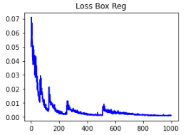
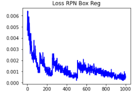
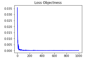
All the metrics from COCO Evaluation are recorded and plotted below.
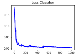
Loss Box Reg Loss RPN Box Reg Loss Objectiveness Loss Classifier
To understand them, refer to COCO’s Detection Evaluation.
True Positive (TP): When the IoU over predicted bounding box and ground truth is greater than or equal to the threshold.
False Positive (FP): When the IoU over predicted bounding box and ground truth is less than threshold.
Average Precision (𝐴𝑃) is the number of true positives in the resulting bounding boxes.
Average Recall (𝐴𝑅) is the proportion of true positives out of possible positives.
COCO Evaluation mentions that they make no distinction between AP and mAP, AR and mAP. The AP and AR are averaged over multiple IoU values. They have used 10 IoU thresholds of .50:.05:.95 (start from 0.5 to 0.95 with a step size of 0.05) instead of computing over a single IoU of .50. Averaging ensures better localization.
The size of objects (area = small, medium, large) is mesasured in number of pixels.
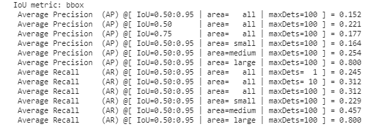
The following can be inferred from the stats of the last iteration:
- The AP @ IoU=0.5:0.95 for area = large is 0.800 which means that when the model detects an object with large area, 80% of the time it matches the ground truth objects.
- The AR @IoU=0.5:0.95 for area = large is 0.800 which means that the model detects 80% of objects with large area, correctly.
- For area = medium and small, the model does not do well. This was probably caused by the small size of dataset and the insufficient number of examples for small and medium sized objects.
The following can be inferred from the loss plots:
- 𝐿𝑜𝑠𝑠 𝐵𝑜𝑥 𝑅𝑒𝑔 is the measure of how tightly the model predicted the bounding box around the true object. It can be observed that the model works well to fit the bbox tightly to the object.
- 𝐿𝑜𝑠𝑠 𝑅𝑃𝑁 𝐵𝑜𝑥 𝑅𝑒𝑔 measures the performance of network for retrieving the region proposals. The plot shows that further training or tweaking the hyperparameters may be required to decrease the loss. This may require more data to improve the results significantly.
- 𝐿𝑜𝑠𝑠 𝐶𝑙𝑎𝑠𝑠𝑖𝑓𝑖𝑒𝑟 measures the performance of the object classification for detected bounding boxes. The plot shows that the model performs well in classifying the objects in the detected bounding boxes.
- 𝐿𝑜𝑠𝑠 𝑂𝑏𝑗𝑒𝑐𝑡𝑛𝑒𝑠𝑠 measures the performance of network for retrieving bounding boxes which contain an object. We can infer that the model is detecting the object very well.
Saving the Model
The model is saved as pickle file and as .pth file with state dictionary so that it can be used later for testing.
#Save the model
torch.save(model, r'./train1000.pkl')

torch.save(model.state_dict(), 'train1000.pth')
torch.save({
    'epoch' : epoch,
    "model_state_dict" : model.state_dict(),
    'optimizer_state_dict' : optimizer.state_dict(),
}, 'ckpt1000.pth')
Saving the Losses and Stats
The loss history and statistics obtained from metric_logger and coco_eval objects are saved for further evaluation. (If unsaved, variables will be lost and the model will have to be trained from the beginning).
#Storing losses and stats in pickle format
import pickle

with open('vars1000.pickle', 'wb') as f:
    pickle.dump([losses, loss_box_reg, loss_rpn_box_reg, loss_classifier, loss_objectness, stat0, stat1, stat2, stat3,
 stat4, stat5, stat6, stat7, stat8, stat9, stat10, stat11], f)
Loading the saved variables
#Load vars pickle file to calc mAP and other statistics.
with open('vars400.pickle', 'rb') as f:
    losses, loss_box_reg, loss_rpn_box_reg, loss_classifier, loss_objectness, stat0, stat1, stat2, stat3,
    stat4, stat5, stat6, stat7, stat8, stat9, stat10, stat11 = pickle.load(f)
Drawing the Bounding Box
The code below obtains the predictions made by the model in the format of a dictionary of boxes, labels and scores.
def showbbox(model, img):
    # The img entered is a tensor in the 0-1 range
    model.eval()
    with torch.no_grad():
        '''
        prediction Like:
        [{'boxes': tensor([[1221.7869,  523.7036, 1272.7373,  575.1018],
        [ 192.8189,  527.5751,  240.7135,  589.8405],
        [ 197.3745,  538.7914,  235.9153,  572.1550],
        [ 195.1216,  533.9565,  238.6585,  578.0548],
        [ 194.0861,  517.0943,  238.0777,  582.4178]], device='cuda:0'),
        'labels': tensor([7, 7, 7, 8, 5], device='cuda:0'),
        'scores': tensor([0.9792, 0.9036, 0.2619, 0.2407, 0.0575], device='cuda:0')}]
        '''
        prediction = model([img.to(device)])

    print(prediction)
    b = prediction[0]['boxes']
    #print(b)
    s = prediction[0]['scores']
    #print(s)

    #Apply Non-maximum suppression:
    keep = torchvision.ops.nms(b,s,0.1)
    #print(keep)

    img = img.permute(1,2,0)  # C,H,W_H,W,C, for drawing
    img = (img * 255).byte().data.cpu()  # * 255, float to 0-255
    img = np.array(img)  # tensor → ndarray
    #Convert np array img to right format.
    img = cv2.cvtColor(img, cv2.COLOR_BGR2RGB)
    #Class number coressponding to Classes
    classes = { 0:' Speed limit (20km/h)' ,
    1:' Speed limit (30km/h)' ,
    2:' Speed limit (50km/h)' ,
    3:' Speed limit (60km/h)' ,
    4:' Speed limit (70km/h)' ,
    5:' Speed limit (80km/h)' ,
    6:' End of speed limit (80km/h)' ,
    7:' Speed limit (100km/h)' ,
    8:' Speed limit (120km/h)' ,
    9:' No passing' ,
    10:' No passing veh over 3.5 tons' ,
    11:' Right-of-way at intersection' ,
    12:' Priority road' ,
    13:' Yield' ,
    14:' Stop' ,
    15:' No vehicles' ,
    16:' Veh > 3.5 tons prohibited' ,
    17:' No entry' ,
    18:' General caution' ,
    19:' Dangerous curve left' ,
    20:' Dangerous curve right' ,
    21:' Double curve' ,
    22:' Bumpy road' ,
    23:' Slippery road' ,
    24:' Road narrows on the right' ,
    25:' Road work' ,
    26:' Traffic signals' ,
    27:' Pedestrians' ,
    28:' Children crossing' ,
    29:' Bicycles crossing' ,
    30:' Beware of ice/snow' ,
    31:' Wild animals crossing' ,
    32:' End speed + passing limits' ,
    33:' Turn right ahead' ,
    34:' Turn left ahead' ,
    35:' Ahead only' ,
    36:' Go straight or right' ,
    37:' Go straight or left' ,
    38:' Keep right' ,
    39:' Keep left' ,
    40:' Roundabout mandatory' ,
    41:' End of no passing' ,
    42:' End no passing veh > 3.5 tons'  }


    for k in range(len(keep)):
        xmin = round(prediction[0]['boxes'][k][0].item())
        ymin = round(prediction[0]['boxes'][k][1].item())
        xmax = round(prediction[0]['boxes'][k][2].item())
        ymax = round(prediction[0]['boxes'][k][3].item())

        label = prediction[0]['labels'][k].item()
        print("Label is: {}\n===\n(Xmin, Ymin, Xmax, Ymax) = ({}, {}, {}, {}) \n===".format(label, xmin, ymin, xmax, ymax))

        #color = list(np.random.random(size=3)*256)
        colors = np.random.uniform(0, 255, size=(43, 3))

        if label in classes:
            pt1 = (xmin, ymin)
            pt2 = (xmax, ymax)
            print("Class Label: "+ classes[label])
            score = prediction[0]['scores'][k].item()
            print("Score: "+ str(score))
            print("\n===============\n")
            color = list(colors[label])
            cv2.rectangle(img, pt1, pt2, color, thickness=2)
            cv2.putText(img, classes[label]+"-"+str(round(score,2)), (xmin, ymin), cv2.FONT_HERSHEY_SIMPLEX, 0.7, color,
                        thickness=2)

    plt.figure(figsize=(40,35))
    plt.imshow(img)

print("Function Loaded"
Non maximum suppression:
A number of proposals can be made by the model for the same object. We can filter the unwanted boxes by using Non-maximum suppression. Torchvision’s library was used to perform NMS.
Next, the Image is converted to the a numpy array from tensor format and then to the RGB format. A dictionary of class ID as keys and values as their string name is declared to display on the image.
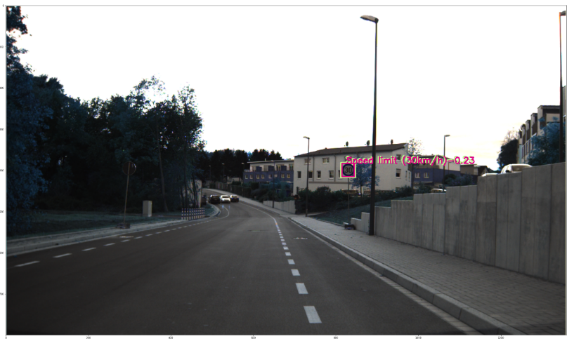
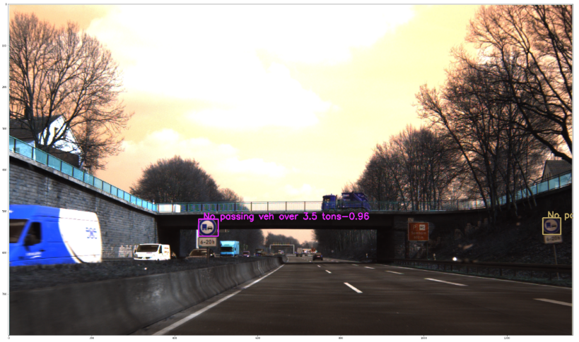
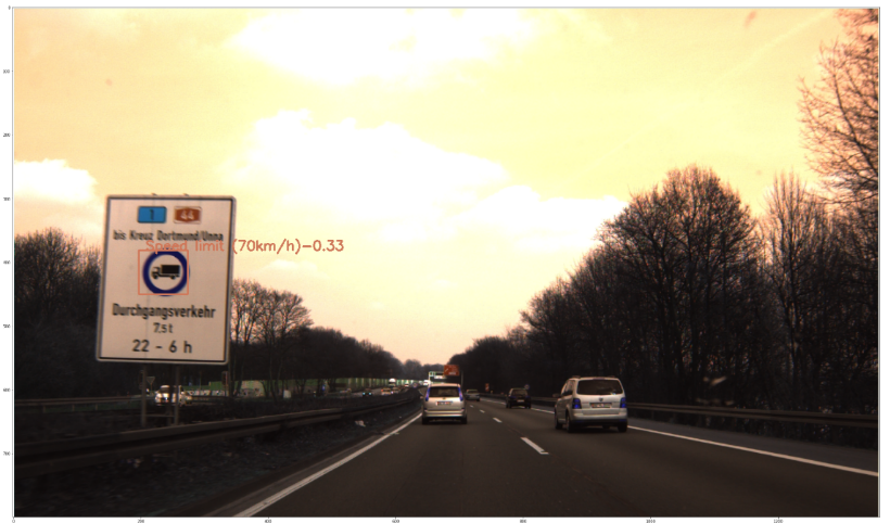
Finally, for every bounding box, a rectangle box and class text is displayed in the predicted image.
Loading the Model from file:
#Load saved model
model1 = torch.load(r'./train400.pkl')
device = torch.device('cuda') if torch.cuda.is_available() else torch.device('cpu')
model1 = nn.DataParallel(model, device_ids=[0,1,2,3])
model1.to(device)
print("Model loaded!")
Testing the Model:
The model has to be tested manually since there were no annotations given for the test set in GTSDB.
#Test the model:
img, _ = dataset_test[99]
showbbox(model, img)
Results
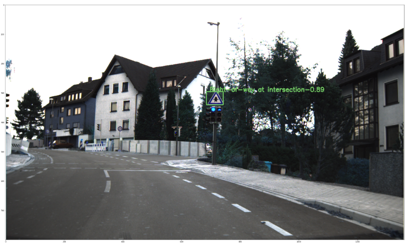
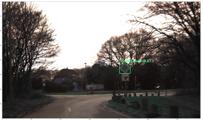
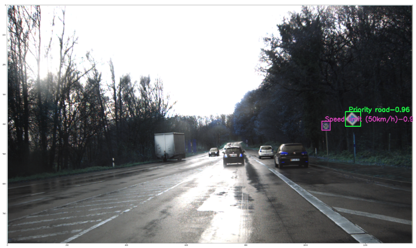
Here are some results:
Results
Compare with other object detection algorithms such as YOLO, SSD, Mask R-CNN, etc.
Create synthetic data using GANs.
Test the model’s performance with video as input.






January 13, 2022 @ 11:28 AM
Hello Mr. Siddharth,
is there any chance that you can send me your pre-trained algorithms.
Sincerely,
Mohamad Barakat
April 22, 2024 @ 4:16 AM
Hello Mr. Siddhart,
is it possible to use my own dataset?
May 22, 2024 @ 9:33 PM
Yes, it is possible to use your own dataset. PyTorch has a great article on writing custom datasets.
https://pytorch.org/tutorials/beginner/data_loading_tutorial.html