Fine-Tuning ResNet50 pretrained on ImageNet for CIFAR-10
Introduction
In this blog post, we will discuss how to fine-tune a pre-trained deep learning model using PyTorch. Fine-tuning is a powerful technique that allows us to leverage the knowledge learned by a pre-trained model on a large dataset and apply it to a new task. This can save a significant amount of time and resources compared to training a model from scratch. The fine-tuned model achieved 92.34% accuracy on the test set.
The CIFAR-10 Dataset
The CIFAR-10 dataset is a widely used dataset for image classification tasks and is a common benchmark for evaluating the performance of deep learning models. The dataset consists of 60,000 32×32 color images in 10 classes, with 6,000 images per class. The classes are: airplane, automobile, bird, cat, deer, dog, frog, horse, ship, and truck. The dataset is split into 50,000 training images and 10,000 test images.
The code provided in this blog post uses the CIFAR-10 dataset to fine-tune the ResNet50 model pre-trained on ImageNet. By using the CIFAR-10 dataset, we can fine-tune the pre-trained ResNet50 model and evaluate its performance on a well-known benchmark dataset, providing a good indication of the model’s generalization ability.
Code
The code structure is explained here. You can find the same code as a jupyter notebook and python file on my Github.
Importing Libraries
Since I find PyTorch very convenient, I use it in most of my computer vision projects. Let’s start by import the libraries we need to run the code.
import torch
import torch.nn as nn
import torch.optim as optim
import torchvision
import torchvision.transforms as transforms
import torchvision.models as models
import matplotlib.pyplot as plt
import numpy as np
import random
Loading the Dataset
Next, we’ll write a function that is responsible for loading the CIFAR-10 dataset, preprocessing the data, and setting up the train and test dataloaders.
The function defines a tuple of classes names corresponding to the 10 classes in the CIFAR-10 dataset, and returns the train and test sets, their respective data loaders and classes.
def load_dataset():
    # Set dataset path
    dataset_path = './data/cifar10'

    transform_train = transforms.Compose([
        transforms.RandomCrop(32, padding=4),
        transforms.RandomHorizontalFlip(),
        transforms.ToTensor(),
        transforms.Normalize((0.4914, 0.4822, 0.4465), (0.2023, 0.1994, 0.2010)),
        ])

    transform_test = transforms.Compose([
        transforms.ToTensor(),
        transforms.Normalize((0.4914, 0.4822, 0.4465), (0.2023, 0.1994, 0.2010)),
        ])


    # Load CIFAR-10 dataset
    trainset = torchvision.datasets.CIFAR10(root=dataset_path, train=True,
                                            download=True, transform=transform_train)
    trainloader = torch.utils.data.DataLoader(trainset, batch_size=32,
                                              shuffle=True, num_workers=2)

    testset = torchvision.datasets.CIFAR10(root=dataset_path, train=False,
                                           download=True, transform=transform_test)
    testloader = torch.utils.data.DataLoader(testset, batch_size=32,
                                             shuffle=False, num_workers=2)

    # Class names for CIFAR-10 dataset
    classes = ('plane', 'car', 'bird', 'cat', 'deer',
               'dog', 'frog', 'horse', 'ship', 'truck')

    return trainset, trainloader, testset, testloader, classes
Training the Model
Once the datasets are loaded and dataloaders are initialized, we can proceed to train the model.
The “train” function is responsible for training the model on the CIFAR-10 dataset. The function performs the training loop for one epoch and returns the updated model parameters, training loss, and training accuracy. It initializes some variables to keep track of the loss and accuracy.
def train(model, trainloader, criterion, optimizer, device):
    train_loss = 0.0
    train_total = 0
    train_correct = 0

    # Switch to train mode
    model.train()

    for inputs, labels in trainloader:
        inputs, labels = inputs.to(device), labels.to(device)

        # Zero the parameter gradients
        optimizer.zero_grad()

        # Forward pass
        outputs = model(inputs)
        loss = criterion(outputs, labels)

        # Backward pass and optimize
        loss.backward()
        optimizer.step()

        # Update training loss
        train_loss += loss.item() * inputs.size(0)

        # Compute training accuracy
        _, predicted = torch.max(outputs, 1)
        train_total += labels.size(0)
        train_correct += (predicted == labels).sum().item()

    # Compute average training loss and accuracy
    train_loss = train_loss / len(trainloader.dataset)
    train_accuracy = 100.0 * train_correct / train_total

    return model, train_loss, train_accuracy
Testing the Model
The “test” function evaluates the model on the test set and returns the test loss and accuracy.
def test(model, testloader, criterion, device):
    test_loss = 0.0
    test_total = 0
    test_correct = 0

    # Switch to evaluation mode
    model.eval()

    with torch.no_grad():
        for inputs, labels in testloader:
            inputs, labels = inputs.to(device), labels.to(device)

            # Forward pass
            outputs = model(inputs)
            loss = criterion(outputs, labels)

            # Update test loss
            test_loss += loss.item() * inputs.size(0)

            # Compute test accuracy
            _, predicted = torch.max(outputs, 1)
            test_total += labels.size(0)
            test_correct += (predicted == labels).sum().item()

    # Compute average test loss and accuracy
    test_loss = test_loss / len(testloader.dataset)
    test_accuracy = 100.0 * test_correct / test_total

    return test_loss, test_accuracy
Iterating the Training
The “train_epochs” function trains the model for specified number of epochs and saves intermediate results. It returns the lists of losses and accuracies for train, and validation sets, which can be used to visualize the training and validation progress and evaluate the performance of the model. This can be used to decide when to stop training, and adjust the hyper-parameters like learning rate, batch size, etc.
def train_epochs(model, trainloader, testloader, criterion, optimizer, device, num_epochs, save_interval=5):
    train_losses = []
    train_accuracies = []
    test_losses = []
    test_accuracies = []

    for epoch in range(num_epochs):
        print(f'Epoch {epoch+1}/{num_epochs}')
        model, train_loss, train_accuracy = train(model, trainloader, criterion, optimizer, device)
        test_loss, test_accuracy = test(model, testloader, criterion, device)

        train_losses.append(train_loss)
        train_accuracies.append(train_accuracy)
        test_losses.append(test_loss)
        test_accuracies.append(test_accuracy)

        print(f'Train Loss: {train_loss:.4f} - Train Accuracy: {train_accuracy:.2f}%')
        print(f'Test Loss: {test_loss:.4f} - Test Accuracy: {test_accuracy:.2f}%')
        print()

        if (epoch + 1) % save_interval == 0:
          # Save the model and variables
          torch.save(model.state_dict(), f'resnet50_cifar10_{epoch+1}.pth')
          checkpoint = {
              'epoch': epoch + 1,
              'train_losses': train_losses,
              'train_accuracies': train_accuracies,
              'test_losses': test_losses,
              'test_accuracies': test_accuracies,
              'classes': classes
          }
          torch.save(checkpoint, f'resnet50_cifar10_variables_{epoch+1}.pth')

    return model, train_losses, train_accuracies, test_losses, test_accuracies
Visualization of Results
To plot the loss and accuracy curves, and display a random image and it’s prediction, we’ll write some utility functions using matplotlib.
def plot_loss(train_losses, test_losses):
    plt.figure()
    plt.plot(range(len(train_losses)), train_losses, label='Training Loss')
    plt.plot(range(len(test_losses)), test_losses, label='Validation Loss')
    plt.xlabel('Epoch')
    plt.ylabel('Loss')
    plt.legend()
    plt.savefig('loss_plot.png')
    plt.show()
def plot_accuracy(train_accuracies, test_accuracies):
plt.figure()
plt.plot(range(len(train_accuracies)), train_accuracies, label='Training Accuracy')
plt.plot(range(len(test_accuracies)), test_accuracies, label='Validation Accuracy')
plt.xlabel('Epoch')
plt.ylabel('Accuracy')
plt.legend()
plt.savefig('accuracy_plot.png')
plt.show()def plot_image(dataset, model, classes):
idx = random.randint(0, len(dataset))
label = dataset[idx][1]
img = dataset[idx][0].unsqueeze(0).to(device) # Move the input image tensor to the GPU
model.eval()
#model.to(device) # Move the model to the GPU
output = model(img)
_, predicted = torch.max(output.data, 1)
# Convert the image and show it
img = img.squeeze().permute(1, 2, 0).cpu() # Move the image tensor back to the CPU and adjust dimensions
plt.imshow(img)
plt.axis('off')
plt.title(f'Predicted: {classes[predicted]}, True: {classes[label]}')
plt.savefig('predicted_image.png')
plt.show()
print("Predicted label: ", classes[predicted[0].item()])
print("Actual label: ", classes[label])Main Function
Finally, to execute the above functions to fine-tune the pretrained ResNet50 on the CIFAR-10 dataset, we will write a main function calling the above defined functions.
Modifying the Pretrained Model
The pretrained ResNet50 model is not directly compatible with the CIFAR10 dataset. This is because the ImageNet dataset has a much larger number of classes than the CIFAR10 dataset. Therefore, we need to modify the pretrained model to suit the CIFAR10 dataset. The final fully connected layer is modified to have 10 output neurons, corresponding to the 10 classes in the CIFAR-10 dataset.
The “conv1” layer in the ResNet50 model from the PyTorch model zoo has a larger kernel size (7×7), stride (2), and padding (3). This configuration reduces the input image size by half at the beginning of the network. This design choice is suitable for the ImageNet dataset, which has larger input image sizes (224×224 pixels). By downsampling the input, the network can capture more global features and patterns from the larger images.
However, for the CIFAR-10 dataset, which has smaller input image sizes (32×32 pixels), this downsampling operation may discard too much information and result in a loss of important details. The reduction in input size early in the network may lead to a significant loss of spatial information and may not be ideal for capturing fine-grained patterns in the smaller images. Therefore, I have modified the network to use a “conv1” layer with a smaller kernel size (3×3), stride (1), and padding (1). This configuration preserves the input size throughout the network. By maintaining the input size, the network can retain more spatial information and capture finer details from the smaller images in the CIFAR-10 dataset. Note that the by retaining the spatial dimensions of the input image, it also means that the subsequent layers may need to handle higher-resolution feature maps, potentially requiring more computational resources.
if __name__ == '__main__':
    # Flag to control whether to run training or use saved fine-tuned model.
    train_model = True

    # Set random seed for reproducibility
    random_seed = 42
    torch.manual_seed(random_seed)
    np.random.seed(random_seed)
    random.seed(random_seed)

    # Number of classes
    num_classes = 10

    # Import ResNet50 model pretrained on ImageNet
    model = models.resnet50(pretrained=True)
    print("Network before modifying conv1:")
    print(model)

    #Modify conv1 to suit CIFAR-10
    model.conv1 = nn.Conv2d(3, 64, kernel_size=3, stride=1, padding=1, bias=False)

    # Modify the final fully connected layer according to the number of classes
    num_features = model.fc.in_features
    model.fc = nn.Linear(num_features, num_classes)
    print("Network after modifying conv1:")
    print(model)

    # Move the model to GPU if available
    device = torch.device("cuda" if torch.cuda.is_available() else "cpu")
    model = model.to(device)

    # Define loss function and optimizer
    criterion = nn.CrossEntropyLoss()
    optimizer = optim.SGD(model.parameters(), lr=0.01, momentum=0.9, weight_decay=5e-4)
    scheduler = optim.lr_scheduler.CosineAnnealingLR(optimizer, T_max=200)

    # Load the dataset
    trainset, trainloader, testset, testloader, classes = load_dataset()

    if train_model:
      # Train the model for 20 epochs, saving every 5 epochs
      num_epochs = 60
      save_interval = 5
      model, train_losses, train_accuracies, test_losses, test_accuracies = train_epochs(
          model, trainloader, testloader, criterion, optimizer, device,
          num_epochs, save_interval)

      # Save the final trained model
      torch.save(model.state_dict(), f'resnet50_cifar10_final_model_epochs_{num_epochs}.pth')

      # Plot and save the loss and accuracy plots
      plot_loss(train_losses, test_losses)
      plot_accuracy(train_accuracies, test_accuracies)
    else:
      # Load the pre-trained model
      model.load_state_dict(torch.load('resnet50_cifar10_final_model_epochs_50.pth'))
      # Load the variables
      checkpoint = torch.load("resnet50_cifar10_variables.pth")
      epoch = checkpoint['epoch']
      train_losses = checkpoint['train_losses']
      train_accuracies = checkpoint['train_accuracies']
      test_losses = checkpoint['test_losses']
      test_accuracies = checkpoint['test_accuracies']
      classes = checkpoint['classes']
      model.to(device)
      model.eval()

    # Plot and save an example image
    plot_image(testset, model, classes)
Hyperparameters
Once we have modified the pretrained model, we can train it on the CIFAR10 dataset. We will use the stochastic gradient descent (SGD) optimizer with a learning rate of 0.01, momentum of 0.9, and a weight decay of 5e-4.
We will train the model for 60 epochs. We will evaluate the model’s performance on the test set after every epoch.
Results
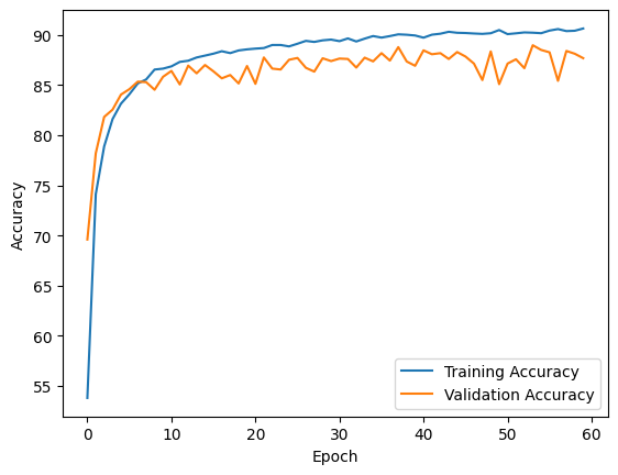
- Training Accuracy: The training accuracy steadily increases with each epoch, starting from 53.80% in the first epoch and reaching 90.64% in the final epoch. This indicates that the model is learning and improving its performance on the training data.
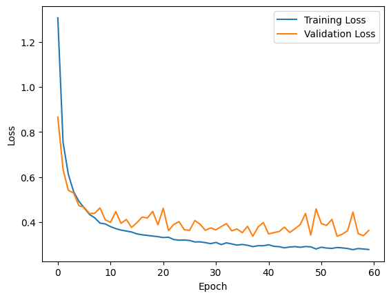
- Training Loss: The training loss gradually decreases over the epochs, starting from 1.3067 and decreasing to 0.2779. Lower training loss values indicate that the model is fitting the training data better.
- Testing Accuracy: The test accuracy also shows improvement throughout the epochs, starting from 69.60% and reaching 87.68% in the final epoch. This suggests that the model is generalizing well and performing better on unseen data.
- Test Loss: The test loss initially decreases and then fluctuates slightly, but overall, it remains relatively stable. It starts at 0.8660 and ends at 0.3625.
Note: Later, I increased the batch size to 64 and I observed a significant increase in training and testing accuracy from 90.64 to 99.51% and 87.68 to 92.34%.
The model shows signs of convergence as the training and test accuracies stabilize and the loss values reach relatively low levels. This indicates that the model has learned as much as it can from the given data and further training may not yield significant improvements.
It’s worth mentioning that achieving high accuracy on CIFAR-10 is a challenging task due to the dataset’s complexity, the small image size (32×32 pixels), and the presence of similar-looking classes.
Conclusion
In this blog post, we explored the process of fine-tuning a pretrained ResNet50 model on the CIFAR-10 dataset. We discussed the code’s functionality, including loading the dataset, training and testing the model, and visualizing the results. By following this example, researchers and practitioners can apply similar techniques to adapt pre-trained models to their specific image classification tasks.
Below are the results for each of the 60 epochs.
Epoch 1/60
Train Loss: 1.3067 - Train Accuracy: 53.80%
Test Loss: 0.8660 - Test Accuracy: 69.60%

Epoch 2/60
Train Loss: 0.7537 - Train Accuracy: 74.12%
Test Loss: 0.6333 - Test Accuracy: 78.20%

Epoch 3/60
Train Loss: 0.6117 - Train Accuracy: 78.88%
Test Loss: 0.5408 - Test Accuracy: 81.82%

Epoch 4/60
Train Loss: 0.5348 - Train Accuracy: 81.61%
Test Loss: 0.5292 - Test Accuracy: 82.55%

Epoch 5/60
Train Loss: 0.4921 - Train Accuracy: 83.14%
Test Loss: 0.4726 - Test Accuracy: 84.05%

Epoch 6/60
Train Loss: 0.4630 - Train Accuracy: 84.08%
Test Loss: 0.4652 - Test Accuracy: 84.59%

Epoch 7/60
Train Loss: 0.4340 - Train Accuracy: 85.16%
Test Loss: 0.4378 - Test Accuracy: 85.34%

Epoch 8/60
Train Loss: 0.4186 - Train Accuracy: 85.56%
Test Loss: 0.4389 - Test Accuracy: 85.29%

Epoch 9/60
Train Loss: 0.3953 - Train Accuracy: 86.55%
Test Loss: 0.4628 - Test Accuracy: 84.53%

Epoch 10/60
Train Loss: 0.3915 - Train Accuracy: 86.64%
Test Loss: 0.4101 - Test Accuracy: 85.82%

Epoch 11/60
Train Loss: 0.3797 - Train Accuracy: 86.86%
Test Loss: 0.3982 - Test Accuracy: 86.41%

Epoch 12/60
Train Loss: 0.3706 - Train Accuracy: 87.31%
Test Loss: 0.4465 - Test Accuracy: 85.06%

Epoch 13/60
Train Loss: 0.3642 - Train Accuracy: 87.42%
Test Loss: 0.3941 - Test Accuracy: 86.94%

Epoch 14/60
Train Loss: 0.3598 - Train Accuracy: 87.75%
Test Loss: 0.4114 - Test Accuracy: 86.17%

Epoch 15/60
Train Loss: 0.3555 - Train Accuracy: 87.94%
Test Loss: 0.3761 - Test Accuracy: 87.00%

Epoch 16/60
Train Loss: 0.3473 - Train Accuracy: 88.13%
Test Loss: 0.3968 - Test Accuracy: 86.37%

Epoch 17/60
Train Loss: 0.3432 - Train Accuracy: 88.37%
Test Loss: 0.4218 - Test Accuracy: 85.67%

Epoch 18/60
Train Loss: 0.3405 - Train Accuracy: 88.18%
Test Loss: 0.4179 - Test Accuracy: 86.00%

Epoch 19/60
Train Loss: 0.3376 - Train Accuracy: 88.45%
Test Loss: 0.4468 - Test Accuracy: 85.16%

Epoch 20/60
Train Loss: 0.3350 - Train Accuracy: 88.56%
Test Loss: 0.3877 - Test Accuracy: 86.90%

Epoch 21/60
Train Loss: 0.3309 - Train Accuracy: 88.63%
Test Loss: 0.4611 - Test Accuracy: 85.12%

Epoch 22/60
Train Loss: 0.3324 - Train Accuracy: 88.69%
Test Loss: 0.3620 - Test Accuracy: 87.75%

Epoch 23/60
Train Loss: 0.3221 - Train Accuracy: 88.99%
Test Loss: 0.3890 - Test Accuracy: 86.64%

Epoch 24/60
Train Loss: 0.3193 - Train Accuracy: 88.99%
Test Loss: 0.4016 - Test Accuracy: 86.55%

Epoch 25/60
Train Loss: 0.3199 - Train Accuracy: 88.85%
Test Loss: 0.3659 - Test Accuracy: 87.52%

Epoch 26/60
Train Loss: 0.3181 - Train Accuracy: 89.12%
Test Loss: 0.3630 - Test Accuracy: 87.70%

Epoch 27/60
Train Loss: 0.3115 - Train Accuracy: 89.40%
Test Loss: 0.4065 - Test Accuracy: 86.72%

Epoch 28/60
Train Loss: 0.3117 - Train Accuracy: 89.30%
Test Loss: 0.3902 - Test Accuracy: 86.34%

Epoch 29/60
Train Loss: 0.3085 - Train Accuracy: 89.46%
Test Loss: 0.3630 - Test Accuracy: 87.67%

Epoch 30/60
Train Loss: 0.3040 - Train Accuracy: 89.53%
Test Loss: 0.3738 - Test Accuracy: 87.39%

Epoch 31/60
Train Loss: 0.3095 - Train Accuracy: 89.38%
Test Loss: 0.3653 - Test Accuracy: 87.64%

Epoch 32/60
Train Loss: 0.2999 - Train Accuracy: 89.65%
Test Loss: 0.3797 - Test Accuracy: 87.60%

Epoch 33/60
Train Loss: 0.3075 - Train Accuracy: 89.34%
Test Loss: 0.3929 - Test Accuracy: 86.74%

Epoch 34/60
Train Loss: 0.3026 - Train Accuracy: 89.63%
Test Loss: 0.3610 - Test Accuracy: 87.73%

Epoch 35/60
Train Loss: 0.2974 - Train Accuracy: 89.89%
Test Loss: 0.3692 - Test Accuracy: 87.36%

Epoch 36/60
Train Loss: 0.3003 - Train Accuracy: 89.73%
Test Loss: 0.3525 - Test Accuracy: 88.18%

Epoch 37/60
Train Loss: 0.2967 - Train Accuracy: 89.88%
Test Loss: 0.3810 - Test Accuracy: 87.44%

Epoch 38/60
Train Loss: 0.2907 - Train Accuracy: 90.06%
Test Loss: 0.3366 - Test Accuracy: 88.78%

Epoch 39/60
Train Loss: 0.2947 - Train Accuracy: 90.02%
Test Loss: 0.3778 - Test Accuracy: 87.35%

Epoch 40/60
Train Loss: 0.2945 - Train Accuracy: 89.94%
Test Loss: 0.3977 - Test Accuracy: 86.92%

Epoch 41/60
Train Loss: 0.2990 - Train Accuracy: 89.72%
Test Loss: 0.3470 - Test Accuracy: 88.46%

Epoch 42/60
Train Loss: 0.2922 - Train Accuracy: 90.02%
Test Loss: 0.3528 - Test Accuracy: 88.07%

Epoch 43/60
Train Loss: 0.2905 - Train Accuracy: 90.12%
Test Loss: 0.3582 - Test Accuracy: 88.18%

Epoch 44/60
Train Loss: 0.2854 - Train Accuracy: 90.31%
Test Loss: 0.3772 - Test Accuracy: 87.60%

Epoch 45/60
Train Loss: 0.2891 - Train Accuracy: 90.21%
Test Loss: 0.3537 - Test Accuracy: 88.29%

Epoch 46/60
Train Loss: 0.2907 - Train Accuracy: 90.19%
Test Loss: 0.3701 - Test Accuracy: 87.84%

Epoch 47/60
Train Loss: 0.2879 - Train Accuracy: 90.14%
Test Loss: 0.3887 - Test Accuracy: 87.14%

Epoch 48/60
Train Loss: 0.2910 - Train Accuracy: 90.10%
Test Loss: 0.4381 - Test Accuracy: 85.50%

Epoch 49/60
Train Loss: 0.2898 - Train Accuracy: 90.17%
Test Loss: 0.3422 - Test Accuracy: 88.35%

Epoch 50/60
Train Loss: 0.2802 - Train Accuracy: 90.48%
Test Loss: 0.4586 - Test Accuracy: 85.09%

Epoch 51/60
Train Loss: 0.2881 - Train Accuracy: 90.08%
Test Loss: 0.3933 - Test Accuracy: 87.14%

Epoch 52/60
Train Loss: 0.2844 - Train Accuracy: 90.16%
Test Loss: 0.3849 - Test Accuracy: 87.57%

Epoch 53/60
Train Loss: 0.2828 - Train Accuracy: 90.25%
Test Loss: 0.4117 - Test Accuracy: 86.68%

Epoch 54/60
Train Loss: 0.2869 - Train Accuracy: 90.22%
Test Loss: 0.3366 - Test Accuracy: 88.97%

Epoch 55/60
Train Loss: 0.2849 - Train Accuracy: 90.17%
Test Loss: 0.3462 - Test Accuracy: 88.50%

Epoch 56/60
Train Loss: 0.2823 - Train Accuracy: 90.43%
Test Loss: 0.3620 - Test Accuracy: 88.26%

Epoch 57/60
Train Loss: 0.2772 - Train Accuracy: 90.58%
Test Loss: 0.4444 - Test Accuracy: 85.42%

Epoch 58/60
Train Loss: 0.2823 - Train Accuracy: 90.38%
Test Loss: 0.3481 - Test Accuracy: 88.40%

Epoch 59/60
Train Loss: 0.2801 - Train Accuracy: 90.41%
Test Loss: 0.3394 - Test Accuracy: 88.12%

Epoch 60/60
Train Loss: 0.2779 - Train Accuracy: 90.64%
Test Loss: 0.3625 - Test Accuracy: 87.68%


