Part 3 – Projected Gradient Descent (PGD)

Welcome to Part 3 of our blog series on Adversarial Machine Learning! In this installment, we will delve into the intricacies of the Projected Gradient Descent (PGD) method—a powerful iterative technique for crafting adversarial examples. We will explore how PGD enhances the Fast Gradient Sign Method (FGSM) by iterating and refining the perturbations, leading to more robust and effective attacks. I will also provide a step-by-step code implementation of PGD using PyTorch and compare the attack success rates of FGSM and PGD.
Projected Gradient Descent (PGD): An Iterative Approach
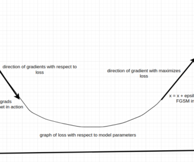
As we’ve learned in our previous post, FGSM is a one step, effective attack method that uses the gradient of the loss function to create adversarial perturbations. However, FGSM has limitations in terms of its perturbation optimization and robustness. PGD, on the other hand, builds upon the principles of FGSM but introduces an iterative refinement process to overcome some of these limitations.
Unlike FGSM where one large step (epsilon) is taken, PGD operates by iteratively applying small perturbations to the input image in a way that maximizes the model’s loss function while staying within a specified perturbation budget, where the adversarial image is clipped in the range of [-epsilon, epsilon]. This iterative nature allows PGD to explore a wider range of perturbations, leading to more sophisticated and potent adversarial examples.
Mathematically, the update rule for PGD can be expressed as:
x_{0}^{adv}=x,\\
x_{t+1}^{adv} = \text{Clip}_{x,\epsilon}\left( x_{t}^{adv} + \alpha \cdot \text{sign}(\nabla_x J(x_{t}^{adv}, y_{true})) \right)
\]
In case of targeted attack, direction is negative gradient with respect to the target class:
x_{t+1}^{adv} = \text{Clip}_{x,\epsilon}\left( x_{t}^{adv} – \alpha \cdot \text{sign}(\nabla_x J(x_{t}^{adv}, y_{target})) \right)
\]
Where:
- \( x_{t}^{adv} \) is the adversarial image at iteration \( t \).
- \( x \) is the clean input image.
- \( \epsilon \) is the \( L_\infty \) perturbation budget.
- \( \alpha \) is the step size.
- \( J \) is the classification loss.
- \( y_{true} \) is the true class label predicted by the model for \( x_{t}^{adv} \).
Clipping Function
The clipping function that performs per pixel clipping of the adversarial image \(X’\) to ensure that the perturbations applied to image are within reasonable bounds to avoid generating unrealistic or visually incoherent images is:
Note: I found this clipping function from “Adversarial Examples in the Physical World“, by Kurakin et. al, that seems to be more accurate and relevant to the objective.
PGD iteratively adjusts the adversarial image by calculating the gradient of the loss function with respect to the current adversarial image and then applying the perturbation scaled by the step size \( \alpha \). The resulting adversarial image is then projected back onto the \( L_\infty \) ball centered at the original image \( x \), ensuring that the perturbations do not exceed the specified budget \( \epsilon \). This process is repeated for a predetermined number of iterations.
Gradient Descent vs Projected Gradient Descent
In the realm of optimization algorithms, Gradient Descent (GD) and Projected Gradient Descent (PGD) stand as crucial techniques for iteratively minimizing functions. While both approaches share similarities, PGD incorporates an additional layer – the concept of projection – to address constrained optimization problems.
Gradient Descent (GD) is a foundational optimization method used to locate the minimum of a given function. Operating on an initial point, GD iteratively adjusts the point in the direction opposite to the gradient of the function, effectively descending toward the optimal solution. However, GD might not be suitable for scenarios with constraints on the solution space, as it can lead to solutions that violate these constraints.
Projected Gradient Descent (PGD), on the other hand, combines GD with the concept of projection to handle optimization tasks in constrained environments. The essence of PGD lies in ensuring that each update adheres to the predefined constraints, making it particularly valuable in scenarios where solutions must satisfy specific conditions.
Projected Gradient Descent = Gradient Descent + Projection.
| Aspect | Gradient Descent (GD) | Projected Gradient Descent (PGD) |
|---|---|---|
| Objective | Minimize function | Minimize function subject to constraints |
| Approach | Unconstrained | Constrained |
| Update Rule | Update: \(x_{k+1} = x_k – \alpha_k \nabla f(x_k)\) | Update: \(y_{k+1} = x_k – \alpha_k \nabla f(x_k),\) Projection: \(x_{k+1} = \text{argmin}_{x \in Q} \frac{1}{2} \|x – y_{k+1}\|^2_2\) |
| Projection | N/A | Enforces constraints |
| Feasibility Guarantee | N/A | Ensures feasible solutions |
| Applicability | Unconstrained | Constrained optimization tasks |
| Computational Complexity | Lower | Potentially higher |
| Solution Convergence | Toward minimum | Toward feasible minimum |
Differences Between FGSM and PGD
- Iterative Nature: The most significant difference between FGSM and PGD lies in their iterative approach. While FGSM applies a single perturbation in one step, PGD applies multiple perturbations iteratively, enhancing its ability to explore the space of possible perturbations.
- Robustness: Due to its iterative nature, PGD-generated adversarial examples tend to be more robust against defenses. By exploring a wider range of perturbations, PGD can craft adversarial examples that are effective against a variety of detection and defense mechanisms.
- Refinement: PGD iteratively refines the perturbations, allowing it to overcome some of the limitations of FGSM. The iterative process enables PGD to generate adversarial examples that are more nuanced and sophisticated.
Implementing Project Gradient Descent (PGD) with PyTorch
Now, let’s dive into the practical implementation of PGD using PyTorch. We’ll use the same ResNet-50 model fine-tuned on CIFAR-10 that we used in our previous post.
The structure of the code is similar to the previous FGSM project. I’ve only replaced the attack function with PGD.
def pgd_attack(model, criterion, images, labels, device, epsilon, alpha, num_iters):
    original_images = images.clone().detach().to(device)
    adversarial_images = images.clone().detach().to(device)

    for _ in range(num_iters):
        adversarial_images.requires_grad_(True)
        outputs = model(adversarial_images)
        loss = criterion(outputs, labels)

        model.zero_grad()
        loss.backward()

        with torch.no_grad():
            gradient = adversarial_images.grad.data
            adversarial_images = adversarial_images + alpha * gradient.sign()

            perturbations = torch.clamp(adversarial_images - original_images, min=-epsilon, max=epsilon)
            adversarial_images = torch.clamp(original_images + perturbations, 0, 1)

        adversarial_images = adversarial_images.detach()
    return adversarial_images, perturbations
- The function is designed to run for a specified number of iterations (
num_iters). - For each iteration, it computes the gradient of the loss w.r.t. the input image, scales it by
alpha, and updates the adversarial image. - Note that the gradients are reset at the beginning of each iteration to calculate the subsequent gradients.
- It applies an upper and lower bound to ensure the perturbations do not exceed
epsilonin any direction. - The adversarial image is clipped to ensure pixel values remain in the range [0, 1].
- After each update, detach() method is used to avoid accumulating gradients from previous iterations.
Results
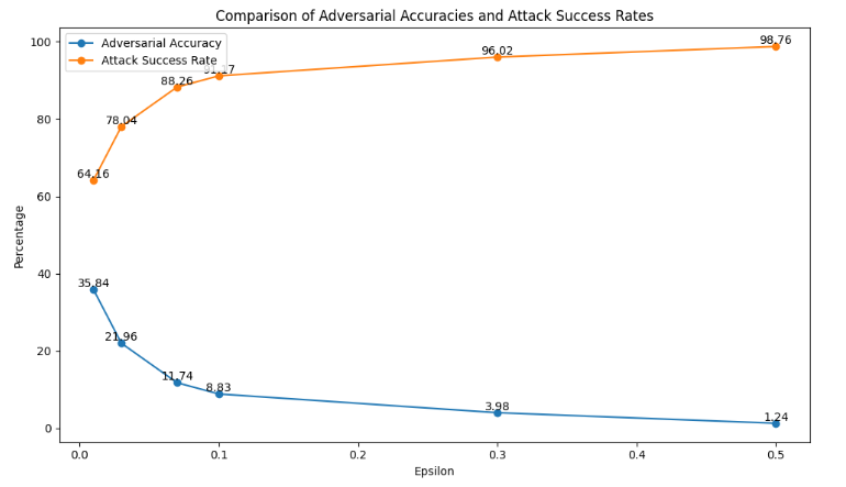
As seen from the results, the model’s adversarial accuracy decreases with increasing epsilon values, while the attack success rate increases correspondingly.

- For an \( \epsilon \) = 0.01, the adversarial accuracy dropped to 35.84%, showing a significant number of successful attacks. With higher epsilon values, the adversarial accuracy decreased sharply, reaching just 1.24% at \( \epsilon \) = 0.5.
- The attack success rate also rose with higher epsilon values, from 64.16% at \( \epsilon \) = 0.01 to 98.76% at \( \epsilon \) = 0.5.
This indicates that the model’s vulnerability to adversarial perturbations increases with larger epsilon values, highlighting the potent nature of the PGD attack.
Analysis and Comparison of FGSM and PGD Attacks
To understand the effectiveness of the FGSM and PGD attacks, we compare their impact on the model’s performance:

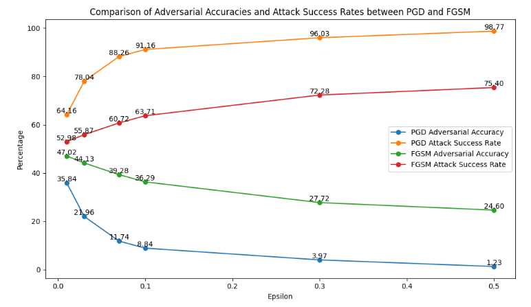
- Adversarial Accuracy: The adversarial accuracy for both FGSM and PGD decreases as the epsilon value increases, but the decline is steeper with PGD. For instance, at epsilon 0.01, FGSM has an adversarial accuracy of 47.02%, whereas PGD achieves only 35.84%. This trend continues with larger epsilon values, highlighting PGD’s greater effectiveness in reducing the model’s accuracy. By epsilon 0.5, FGSM’s adversarial accuracy is 24.60%, while PGD’s is drastically lower at 1.23%.
- Attack Success Rate: The attack success rate for both FGSM and PGD increases with higher epsilon values, indicating that both attacks become more successful at fooling the model with stronger perturbations. However, PGD consistently achieves a higher attack success rate compared to FGSM. For example, at epsilon 0.01, FGSM’s success rate is 52.98%, while PGD’s is 64.16%. This gap widens with larger epsilon values, with FGSM achieving a success rate of 75.40% at epsilon 0.5, compared to PGD’s 98.77%.
Effect of Epsilon (\( \epsilon \)) on Adversarial Image
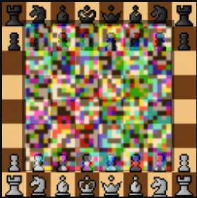
- Magnitude of Pertubations Increases: As \( \epsilon \) increases, the magnitude of the perturbations becomes larger. The changes to the pixel values become more significant, making the perturbations noticeable.
- Image Quality Degradation: Higher values of \( \epsilon \) causes noticeable artifacts in the image. The image starts looking noisy or distorted as the perturbations grow larger.
- Pixel Values Saturation:
- Small \( \epsilon \) : Pixels are altered slightly within their value range (e.g., [0, 255] for 8-bit images).
- Large \( \epsilon \) : As \( \epsilon \) increases, it becomes more likely that the perturbed pixel values will reach the maximum or minimum possible values (e.g., 0 or 255), causing a saturation effect where further perturbations do not change the pixel value.
\( \epsilon \) = 0.01


\( \epsilon \) = 0.03


\( \epsilon \) = 0.07


\( \epsilon \) = 0.01


\( \epsilon \) = 0.3


\( \epsilon \) = 0.5


Conclusion
In this blog post, we delved into the mechanics of the Projected Gradient Descent (PGD) attack, a powerful and iterative technique that enhances the Fast Gradient Sign Method (FGSM) by applying multiple small perturbations to create more effective adversarial examples. By iteratively refining the perturbations and projecting the adversarial images back within the allowable perturbation budget, PGD generates sophisticated attacks that significantly decrease the model’s accuracy, as demonstrated by our results using a ResNet-50 model on CIFAR-10.
Our analysis showed that PGD outperforms FGSM in terms of reducing adversarial accuracy and increasing the attack success rate, particularly as the perturbation budget (\( \epsilon \)) increases. FGSM, while still effective, does not reduce the model’s adversarial accuracy as dramatically as PGD.


